E-stop circuit

This is the E-stop circuit I am going to use when upgrading the cnc-mill to servo control. The idea is to use a wire-OR circuit (series connection of NC switches) for things that cause an E-stop followed by a wire-AND circuit (parallel connection of relays) for things I want to happen at E-stop.

The E-stop out signal from EMC is wired to the top right of this board (labeled E-stop IN...). When this signal goes high it closes the rightmost relay which has +12V wired to it. The 12 V then goes through a series of NC switches, which I've here just shorted out with the black wires. In reality the black wires will be replaced by one E-stop button on the main enclosure, one E-stop button on the jog-pendant, X/Y/Z limit switches, NC servo-amp fault relays, and a VFD NC fault relay.

When all is well +12 V is supplied to the three other relays, and these provide NC or NO outputs. One is used to tell EMC everything is OK (E-stop IN signal in EMC), one is used to enable the power switch of the axis servos, and one is spare for now.

This should make the machine reasonably safe. If any of the E-stop buttons are pressed, a limit is tripped, or the servo amps/VFD are not feeling well we should go into E-stop, and that will cut power from the servos. EMC will also notice this and I'm relying on EMC to shut down the coolant pump and the VFD.

Barlow test

The big picture shows a normal photo through an f=1000mm F/9.8 telescope with a Canon 20D. The field of view should be around 1° 17‘ 20" according to this FOV calculator. The small frame is taken with an additional 2x Barlow lens between prime focus and the camera sensor. It ends up magnifying the image around 2.7- to 2.9-fold. I guess this could be tuned a little each way by inserting the Barlow differently in the focuser or with a T-ring standoff between the camera and the Barlow.

Something to try on the moon or bright planets once the skies are clear again...

Saturn

Had hoped to shoot the Pleiades with some longer exposures today, but clouds rolling in prevented that. So some snapshots at ISO100 and 1/4s of Saturn instead. These are 100% crops, so maybe I need to get an adapter for eyepiece-photography for shooting planets at higher magnification?

The clouds caused this round halo-effect around the moon. By 23:00 it was impossible to shoot stars.

Moon photo

Pooling our hardware resources together in the lab, we now have a 102 mm F/9.8 (f=1000 mm) refractor on an EQ6 equatorial mount and either a Canon 20D or a Canon 400D to shoot with. When one camera is coupled to the scope the other one can simultaneously take a wide-field photo. Did not bother with polar-aligning the mount today, so just looked visually at the moon, mars (it happened to be close to the moon), and M42. The moon is so bright no tracking is really needed.

Here is the moon through a 102mm F/9.8 (f=1000mm) refractor with a Canon 400D at prime focus, set to ISO400 and 1/160s. Around 21:40 local time on Friday 15 Feb 2008.

Astrophotography in Finland is a cold hobby, I was somewhat unprepared for the weather so around 60 min in -7 C was enough for me...

Z-map model for 3-axis machining

I've been reading about the z-map model for 3-axis milling. A working simulation environment would be very useful for CAM algorithm development. Coarse errors in the algorithms can be spotted by eye from the simulation, and a comparison of the z-map with the original CAD model can be used to see if the machining really produces the desired part within tolerance.

Jeff Epler hacked together a z-map model with EMC2 a while ago: gdepth. Perhaps some code/ideas can be borrowed from there.

The z-map can also be used for generating the tool paths themselves (similar to bitmap-mowing here, here and here), but that's more advanced and not the immediate goal.

Here's the z-map model, a lot of vectors standing upright in the z-direction, getting cut (or mowed down) by the moving tool. For graphics you could fill each space between four z-vectors with two triangles and display an STL surface. Obviously this works only for 3-axis machining where the tool is oriented along the z-axis, and the tool must also not produce undercuts (e.g. T-slot milling).

So how do you cut down the z-vectors for each move in the program? For linear moves you can always rotate your coordinate system so it looks like the figure above. The movement is along the x axis, with possibly a simultaneous move in the z-axis. At the beginning of each move (A) and at the end (C) it's very simple, you just calculate the intersection of the relevant z-vectors with a stationary tool at A and C, a kind of 'inverse drop-cutter' idea.

The surface the tool sweeps out during the move itself (B) is more difficult to deal with. The mathematics of the swept surface leads to an equation which most people seem to solve numerically by iteration. I'd like to go through the math/code in a later post (need to learn how to put equations in posts first!).

It's not smart to test all z-vectors in the model against the tool envelope of each move. So like drop-cutter where you are searching for which triangles are under the tool, in z-map you want to know which z-vectors are under the tool envelope. One strategy is simple bucketing, but perhaps if a kd-tree is developed for drop-cutter the same algorithm can be used for z-map.

Obviously the z-map has a finite resolution. Increasing the linear resolution by some factor a requires a^2 more z-vectors, storage, and calculations. A better way might be to insert more z-vectors only where they are needed. That's the places on the model where the z-coordinate changes a lot. So here (view from above) for example if you are milling with a cylindrical cutter more z-vectors are needed along the edge of the tool envelope. (I have no idea why they are inserted in a tilted grid-pattern in the above figure...). This potentially leads to much reduced memory/calculation requirements, while still producing a high resolution model. As the simulation progresses there are probably also regions where some densely spaced z-vectors could be removed. Maybe a 'garbage-collector' process could go over the model every now and then and look for flat areas (xy-plane like regions) where less z-vectors are needed and remove them.

A lot of papers use this APT tool when deriving the equations for machining or simulations. By varying the parameters suitably you get the familiar tool shapes below:

From left to right: Bull-nose/filleted/toroidal, Round/ball-nose/spherical, drill/countersink, tapered, and cylindrical.

My earlier drop-cutter explanations and code only work with the toroidal, spherical, and cylindrical cutters. I'm not sure if it makes sense to write the code for the general APT cutter, or if it's better to optimize for each case (cylindrical and spherical are usually quite easy).

If anyone has made it this far, my sources are the following papers - which are available from me if you ask nicely by email.

Helsinki Boatshow 2008

The 2008 Helsinki Boatshow started yesterday with a day for press and other VIPs. Four Micro-Magic boats were sponsored by the Finnish Sailing Federation and its parters, and on Friday a few of the Finnish Olympic sailors got together for some racing in the pool. The show is now open until Sunday 17th, and the Finnish Micro-Magic sailors are sailing in the pool 2-3 times per day for 30 minutes at a time. This pool is a bit smaller, 4.5x9.5 m, than the one at Model Expo last year, but we found some better fans for generating wind. They seem to create less turbulence and a smoother wind across the pool.

Widgets for Sail

Graham Elliot from the UK doesn't have a website of his own (yet?) , but wanted to let everyone know that he is now building and selling the Widget IOM. Designed by Chris Dicks in 1995 the boat has gone through quite a few changes to everything except the hull shape. The Widget has won the 1996 European Championship, the British National championships in 1997 and 2007, and the 2007 World Championship, not bad for a boat that was designed 13 years ago. The mouldings of the boat are manufactured by Dave Creed.

Graham's options and prices are:

  • Boat complete to deck level, including cf fin and rudder, all attachment points, pulleys, adjustable main post, keel, all finished = 840 euro.
  • RMG 280D, 42mm drum, thumbscrew, fitted in boat=215 euro.
  • Rudder Servo, hitec 645 ultra torque, fitted in boat=75 euro.
  • Rigs: prices vary depending on which fittings (sails etc or housemartin) and also which sails are preferred (housemartin , Brad Gibson , Stealth , sails etc)
  • Wooden rig box= 80 euro
  • 4 colours: red, orange, blue, grey. They are all sprayed using Epifanes 2 pot polyurethane paint.

Currently (Feb 2008) there is a waiting list of approximately 16-18 weeks.

Please contact Graham Elliot on elliottyachts "at" hotmail.co.uk if you are interested!

Mowing Foam

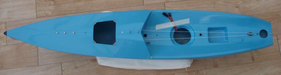
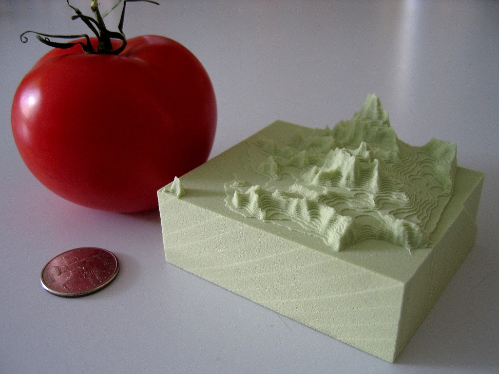
Dan Egnor sent me this nice example of bitmap-based toolpath generation, or 'pixel mowing'. It's a slightly exaggerated topographic relief of San Francisco machined in tooling board using a very simple 'lawn mowing' toolpath generator.

The explanation of how it works below is mostly Dan's, not mine.

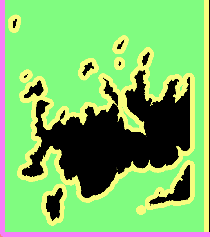
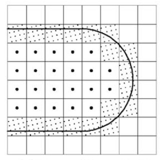
This is the input to the toolpath generator for one of the Z-slices.

black - material which must not be touched
green - to be removed, is safe (at least one tool radius from black)
yellow - remove if possible, is dangerous (within tool radius of black)
purple - has been cleared, is dangerous (machine limits or similar)
white - has been cleared, is safe, is not blue (below)
blue - this spot has been cleared, and is safe, but is within one tool radius of material that needs clearing (green or yellow)

Note that you don't see blue in either "before" or "after" images, it only occurs transiently. (In theory it could show up in "before" as area outside the workpiece.)

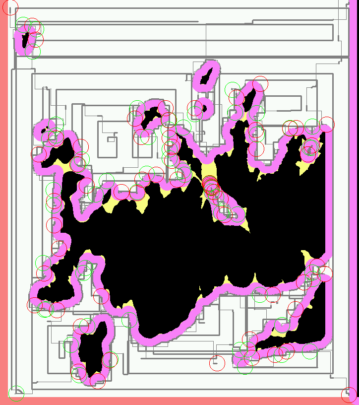
And this is the resulting toolpath. Green circles are plunges and red circles are lifts. The thick grey lines represent actual cuts, the thinner lines are rapid feeds.

The basic rule is that the tool *centroid* is only allowed to visit safe areas (green, blue, and white). Green and blue represent work to be done (safe areas that need visiting). Of course, as the tool moves, green changes to blue and white, and (some) yellow changes to purple.

The real trick is in efficiently tracking the "within tool radius of" zones (material to be cut, or material to stay away from). Every pixel keeps a count of how many pixels of each type ("nearby-blocking" or "nearby-cutting") are within one tool radius of that pixel. Whenever a value is changed ( e.g. the simulated tool moves and changes some points from "cut" to "clear"), every counter within the appropriate radius is updated.

That would be rather costly to implement directly, each simulated pixel move would require N^3 updates, if N is the diameter of the tool. Instead those counters are only kept as *differences* between each point and its neighbours. That means changing a point only requires updating the values along the *perimeter* of the radius surrounding that point, meaning that a simulated pixel move only requires N^2 updates, which makes things a lot more tractable (though it still takes the old laptop I use a couple minutes to complete the toolpaths for a 5" x 3" x 1.5" model at 1/256" resolution). Of course this means that the "color state" isn't directly accessible for a random pixel, but must be figured incrementally from neighboring values. Fortunately most operations don't access random pixels.

You would probably not want to cut metal with this kind of algorithm as there is no control over material removal rate or cutting forces, but for foam, tooling-board, or wood it should work ok.

Dan's program is written in C++ and available here (http://svn.ofb.net/svn/egnor/boring/), but it's not well documented.

We are standing by for a video of this kind of cutting!