Sliptonic has worked on connecting FreeCAD with OpenVoronoi to produce V-carving (aka medial-axis) toolpaths.
I worked on the OpenVoronoi stuff 7 years ago and we made this video back then:
Sliptonic has worked on connecting FreeCAD with OpenVoronoi to produce V-carving (aka medial-axis) toolpaths.
I worked on the OpenVoronoi stuff 7 years ago and we made this video back then:
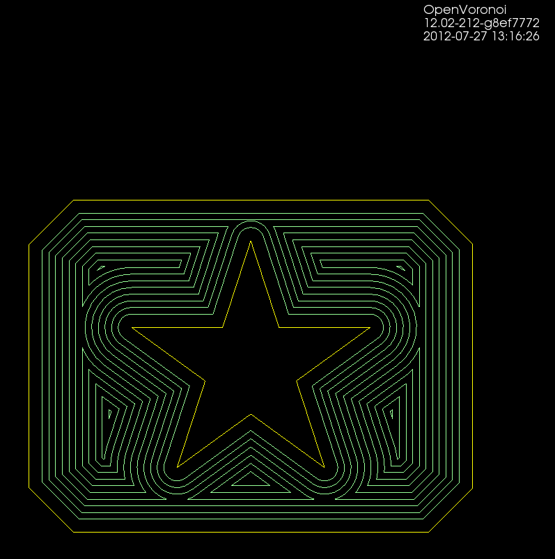
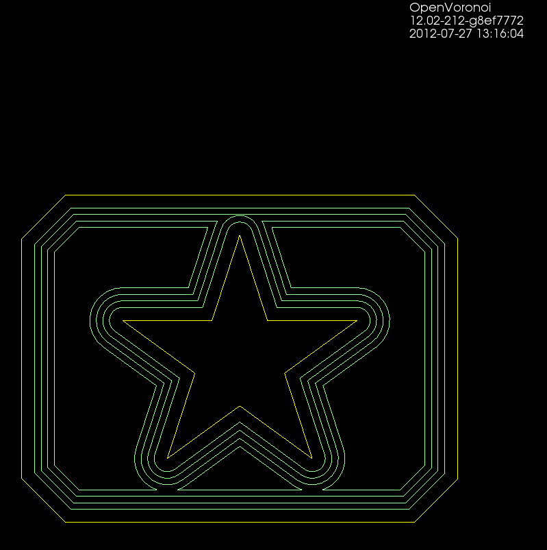
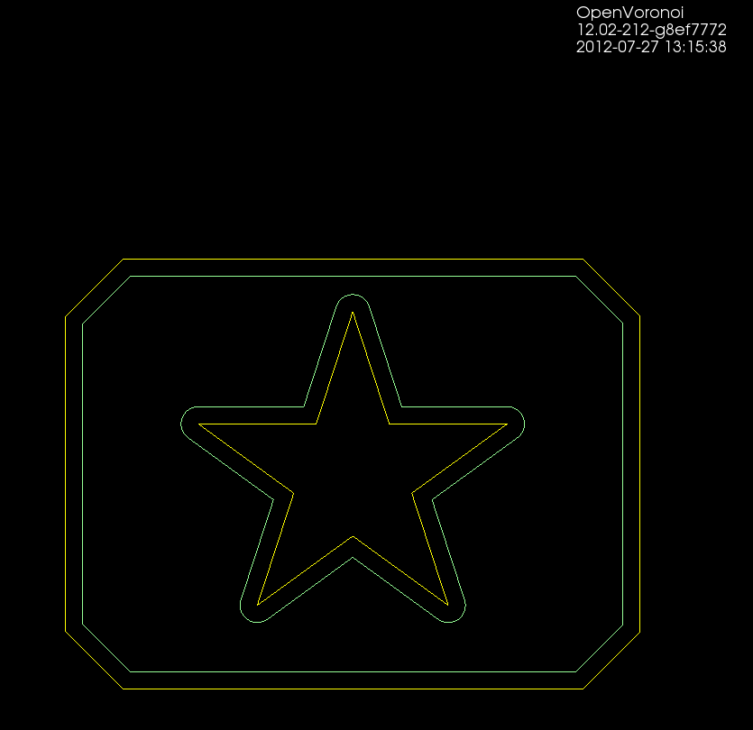
Some basic pocketing loops generated on the train today.
Using pycam's revise_directions() function it is possible to clean up the DXF data and classify polygons into pockets and islands.
There's a new parameter N_offsets
N_offsets=1 generates just a single offset at a specified offset-distance.N_offsets=2... generates the specified number of offsets. Possibly with an increment in offset-distance that is not equal to the initial offset-distance. This happens e.g. when we want the final pass of the tool to be one cutter-radius from the input geometry but the material is difficult to machine and we want the "step-over" for interior offset-loops to be less than the cutter-radius.N_offsets=-1 produces a complete interior pocketing path. Offsets are first generated at the initial offset distance and successive offsets are then generated at increasing offset distance until no offset-output is generated.
Todo: Nesting, Linking, Optimization.
There's no nesting among the loops here. The algorithm will have no clue in what order to machine the offset loops. A naive approach is to machine all loops at the maximum offset distance, then move one loop outwards, etc. But this is clearly not good as the tool would jump between the growing pockets during machining. Nesting information should be straightforward to extract from the voronoi diagram during offset-generation. The nested loops form a tree/graph, which we traverse in some suitable order to machine the entire pocket.
Also, there is no linking of these loops to eachother. For a machining toolpath one wants to link the offsets to each other so that the tool can be kept down in the material when we move from one offset loop to the next. A simple algorithm for linking should be straightforward, but I suspect something more involved is required to prevent overcutting with sufficiently complex input geometry.
When one has nested and linked offset paths, in general there still will remain "pen-up", "rapid traverse", "pen down" transitions. An asymmetric TSP solver could be run on this to minimize the rapid traverse distance (machining time).
A very early result with trying to use openvoronoi from pycam:

Pycam reads the geometry from a DXF file, does some pre-processing of the geometry, pushes it over to openvoronoi which computes a VD and the offsets. Offsets (line-segments and arcs) are then communicated back to pycam for display and g-code generation.
Here's some benchmark data for constructing the Voronoi diagram (or its dual, the Delaunay triangulation) for random point sites. Code for this benchmark is over here: https://github.com/aewallin/voronoi-benchmark

OpenVoronoi is my own effort using the incremental topology-oriented algorithm of Sugihara&Iri and Held. Floating-point coordinates with all sites falling within the unit-circle are used. Fast double-precision arithmetic is used for geometric predicates (e.g. "in-circle") during the incremental construction of the diagram, since the topology-oriented approach ensures that the algorithm finishes and produces an output graph regardless of errors in the geometric predicates. Quad-precision arithmetic is used for positioning vd-vertices. This benchmark runs in ca 7us*N*log2(N) time.
Boost.Polygon uses Fortune's sweepline algorithm. Only integer input coordinates are allowed, which ensures that geometric predicates can be computed exactly. Lazy arithmetic, where a high-precision slower number-type is used only when required, is used. This benchmark runs in ca 0.2us*N*log2(N) time.
CGAL uses exact geometric computation, which is slow but supposedly robust. The run-time gets worse with increasing problem-size and doesn't seem to fall on an O(N*log(N)) line.
Some thoughts:
I started working on arc-sites for OpenVoronoi. The first things required are an in_region(p) predicate and an apex_point(p) function. It is best to rapidly try out and visualize things in python/VTK first, before committing to slower coding and design in c++.
in_region(p) returns true if point p is inside the cone-of-influence of the arc site. Here the arc is defined by its start-point p1, end-point p2, center c, and a direction flag cw for indicating cw or ccw direction. This code will only work for arcs smaller than 180 degrees.
def arc_in_region(p1,p2,c,cw,p): if cw: return p.is_right(c,p1) and (not p.is_right(c,p2)) else: return (not p.is_right(c,p1)) and p.is_right(c,p2) |

Here randomly chosen points are shown green if they are in-region and pink if they are not.
apex_point(p) returns the closest point to p on the arc. When p is not in the cone-of-influence either the start- or end-point of the arc is returned. This is useful in OpenVoronoi for calculating the minimum distance from p to any point on the arc-site, since this is given by (p-apex_point(p)).norm().
def closer_endpoint(p1,p2,p): if (p1-p).norm() < (p2-p).norm(): return p1 else: return p2 def projection_point(p1,p2,c1,cw,p): if p==c1: return p1 else: n = (p-c1) n.normalize() return c1 + (p1-c1).norm()*n def apex_point(p1,p2,c1,cw,p): if arc_in_region(p1,p2,c1,cw,p): return projection_point(p1,p2,c1,cw,p) else: return closer_endpoint(p1,p2,p) |

Here a line from a randomly chosen point p to its apex_point(p) has been drawn. Either the start- or end-point of the arc is the closest point to out-of-region points (pink), while a radially projected point on the arc-site is closest to in-region points (green).
The next thing required are working edge-parametrizations for the new type of voronoi-edges that will occur when we have arc-sites (arc/point, arc/line, and arc/arc).
My first attempt at MA-pocketing only worked when the medial axis of the pocket was a tree (a connected acyclig graph).

I've now extended this to work with pockets consisting of many parts which ha a MA consisting of multiple connected components. There's also simple support for when the MA has cycles, such as seen in "P" and "O" above. With a large cut-width the toolpath looks like this:

Each component of the pocket starts at the red dot with a pink spiral that clears the largest MIC of the pocket. The rest of the pocket is then "scooped out" using green cut-arcs connected with cyan (tool down) or magenta (tool up, at clearance height) rapid moves.
Instead of clearing the interior of letters we can also clear a pocket around the letters. The MA then looks like this:

This video shows quite a lot of "air-cutting". This is because the algorithm only keeps track of the previously cleared area behind the MIC that is currently being cleared. When we come to the end of a cycle in the MA the algorithm does not know that in fact MICs in front of the current MIC have already been cleared.
Update: In the US, where they are silly enough to have software-patents, there's US Patent number: 7831332, "Engagement Milling", Filing date: 29 May 2008, Issue date: 9 Nov 2010. By Inventors: Alan Diehl, Robert B. Patterson of SURFWARE, INC.
Any pocket milling strategy will have as input a step-over distance set at maybe 10 to 90% of the cutter diameter, depending on machine/material/cutter. Zigzag and offset pocketing paths mostly maintain this set step-over, but overload the cutter at sharp corners. Anyone who has tried to cnc-mill a hard material (steel) using a small cnc-mill will know about this. So we want a pocketing path that guarantees a maximum step-over value at all times. Using the medial-axis it is fairly straightforward to come up with a simple pocketing/clearing strategy that achieves this. There are probably many variations on this - the images/video below show only a simple variant I hacked together in 2-3 days.
The medial-axis (MA, blue) of a pocket (yellow) carries with it a clearance-disk radius value. If we place a circle with this radius on the medial-axis, no parts of the pocket boundary will fall within the circle. If we choose a point in the middle of an MA-edge the clearance-disk will touch the polygon at two points. If we choose an MA-vertex of degree three (where three MA-edges meet), the clearance-disk will touch the pocket at three points.
MA-pocketing starts by clearing the largest clearance-disk using a spiral path (pink).

From the maximum clearance-disk we then proceed to clear the rest of the pocket by making cuts along adjacent clearance-disks. We move forward along the MA-graph by an amount that ensures that the step-over width will never be exceeded. The algorithm loops through all clearance-disks and connects the arc-cuts together with bi-tangents, lead-out-arcs, rapids, and lead-in-arcs.

This video shows how it all works (watch in HD!). Here the cutter has 10mm diameter and the step-over is 3mm.
I'll try to make a variant of this for the case where we clear all stock around a central island next. These two variants will be needed for 3D z-terrace roughing.
Update: some work on connecting MICs together with bi-tangent line-segments, as well as a sequence of lead-out, rapid, lead-in, between successive MIC-slices:

It gets quite confusing with all cutting and non-cutting moves drawn in one image. The path starts with an Archimedean spiral (pink) that clears the initial largest MIC. We then proceed to "scoop" out the rest of the pocket with circular-arc cutting moves (green). At the end of a scoop we do a lead-out-arc (dark blue), followed by a linear rapid (cyan), and a lead-in-arc (light blue) to start the next scoop.
Next I'd like to put together an animation of this. The overall strategy will be much clearer from a movie.
This animation shows MICs, i.e. maximal inscribed circles (green, also called clearance-disks), inside a simple polygon (yellow). The largest MIC is shown in red.
This is work towards a new medial-axis pocketing strategy. The largest MIC (red) is first cleared using a spiral strategy. We then proceed to clear the rest of the pocket in the order that the MICs are drawn in the animation. We don't have to spin the tool around the whole circle. only the parts that need machining, which is the part of the new MIC that doesn't fall inside the previously machined MIC. As mentioned in my previous post this is inspired by Elber et al (2006).
The next step is to calculate how we should proceed from one MIC to the next, and how we do the rapid-traverse to re-position the tool for the next cut.
See also the spiral-toolpath by Held&Spielberger (2009) or their 199-slide presentation. The basics of this spiral-strategy is a straightforward march along the medial-axis. But then a filtering/fitting algorithm, which I don't have at hand right now, is applied to get the smoothed spiral-path.
Update: Here is "VX" with FreeSerifItalic. There is overlap in LibreOffice also.

For the most part truetypetracer produces valid and nice input data for testing openvoronoi. But sometimes I see wiggles, and now this:

It is frustrating to try to track down bugs in downstream algorithms that take this as input, and assume all line-segments are non-intersecting when in fact the are not!
I seem to have only 13 .ttf files in my /usr/share/fonts/truetype/freefont folder, but maybe there are more elsewhere. I should find a font that is properly designed without wiggles and without overlaps. The other approach is to write a pre-processor that looks at input data and either rejects or cleans it. Looking for all pair-wise intersections of N line-segments is a slow N^2 algorithm - at least for a naive implementation (without bounding-boxes or binning or other tricks).
Unlike the wiggles, this overlap doesn't happen in Inkscape:

Here is G-code generated with ttt-4.0 and drawn in LinuxCNC:

Here is a screenshot from LibreOffice 3:

and GIMP:

A first try at v-carving, with toolpaths produced by the ttt2medial python script.
