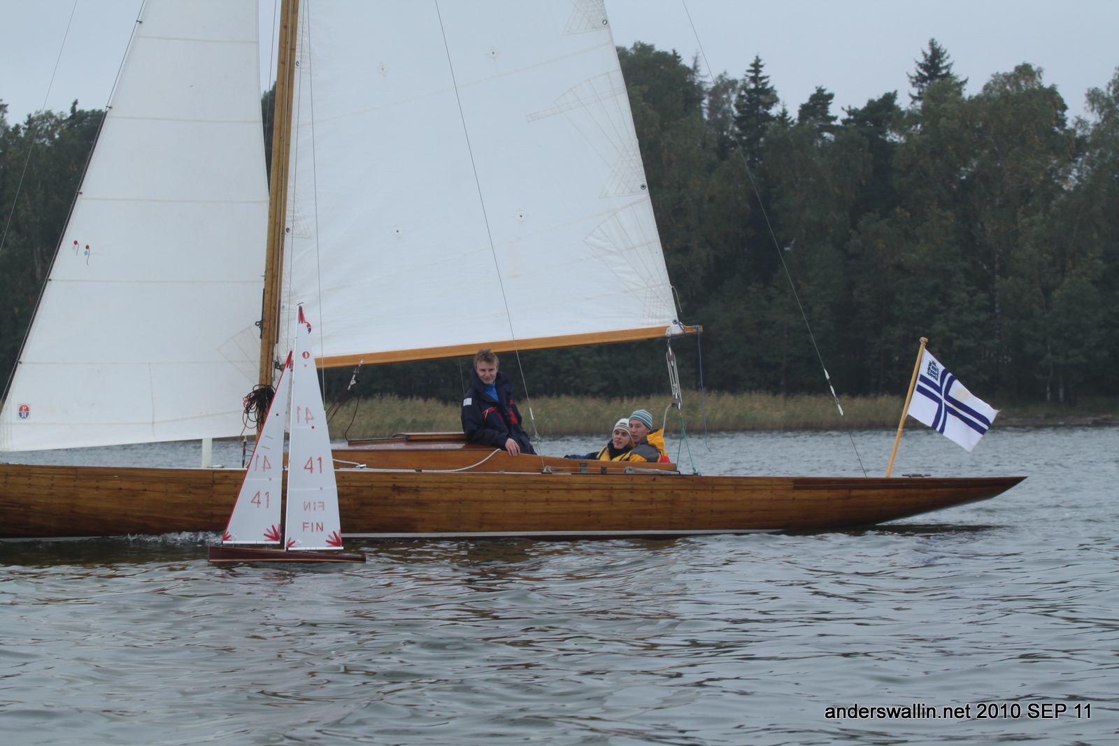
Proof that Stockholm is much closer to the Center of The World than Helsinki:
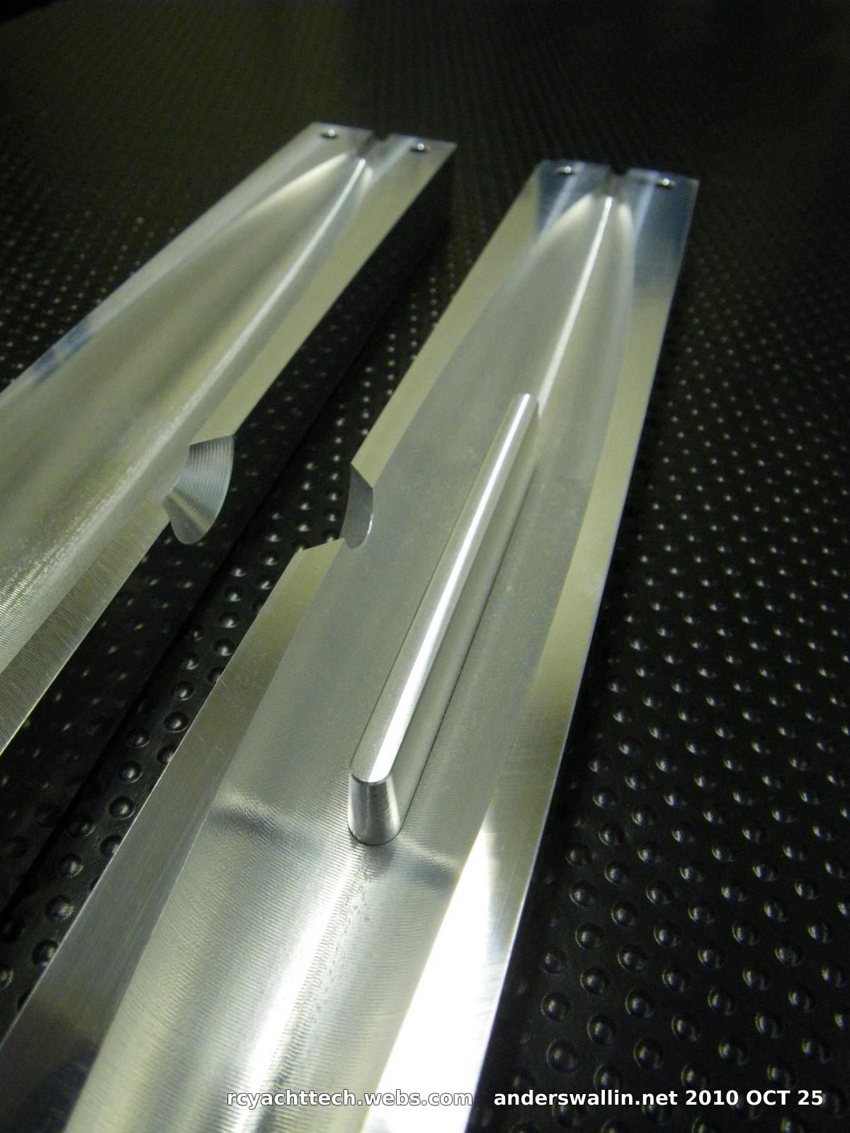
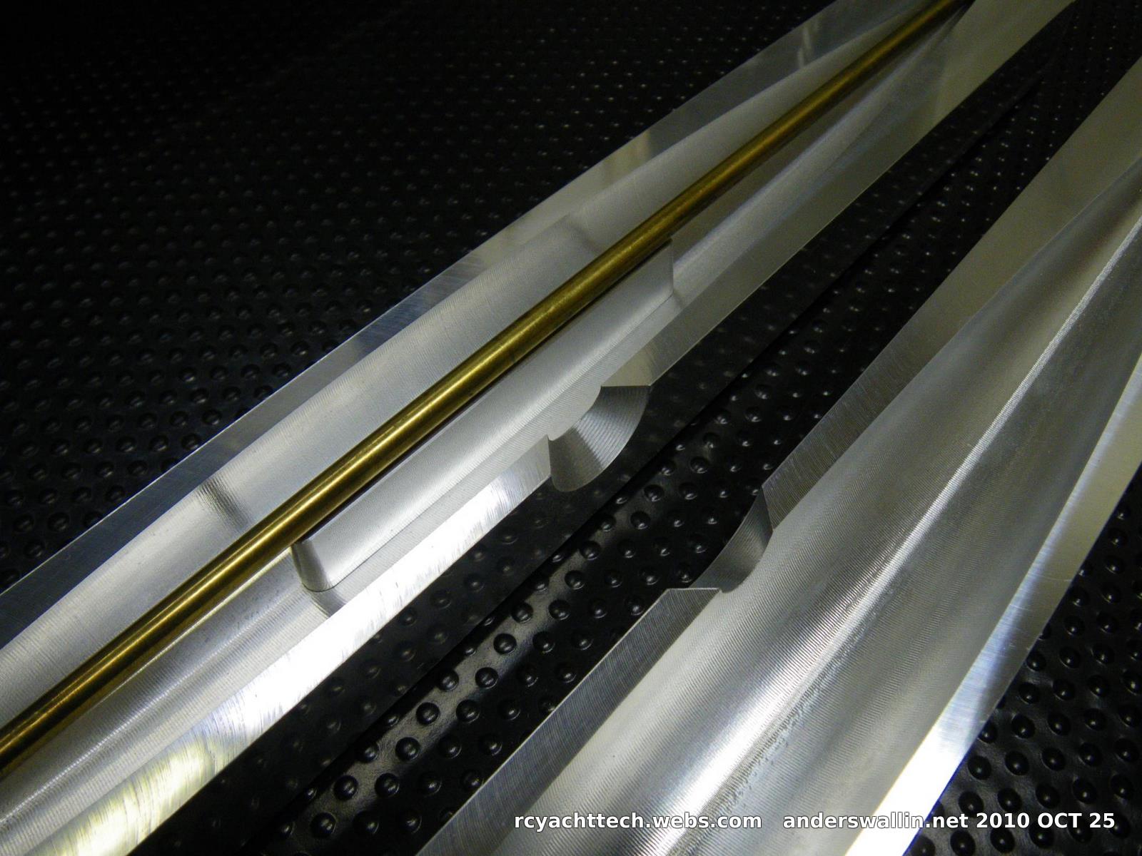
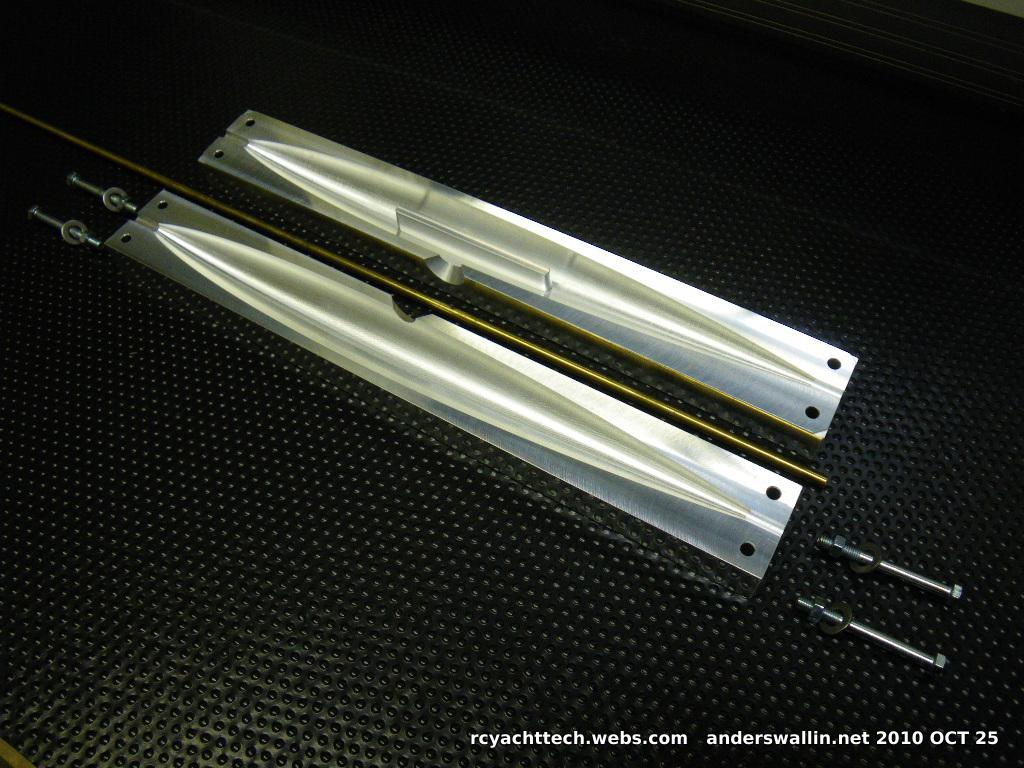
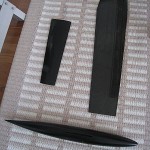
Jari made these new IOM bulb-moulds over the weekend. CNC-milled in aluminium. Circular cross-section with a NACA0010-34 profile (similar to my 2005 design), length ca 360mm. Designed with a central stiffening brass rod. Check out rcyachttech.webs.com for more cnc-machined moulds and parts.
See also casting notes from 2003.
Update2: youtube-videos
Update: final results: http://www.rc-purjehdus.net/2010/09/2010-iom-nordic-championships-%E2%80%93-day-2/
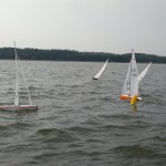
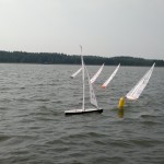
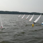
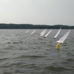
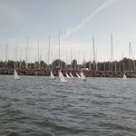
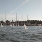
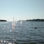
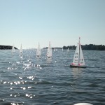
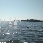
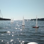
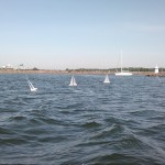
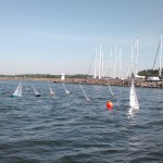
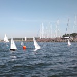
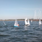
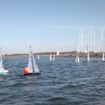
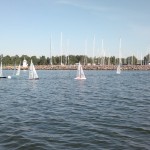
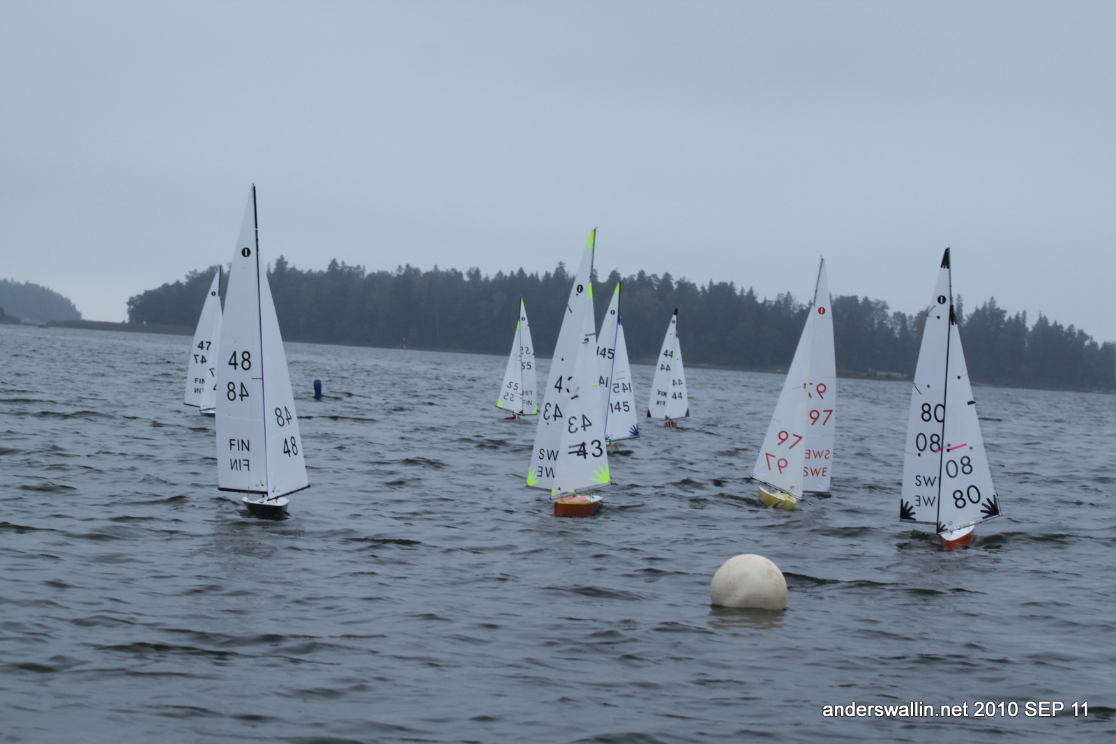
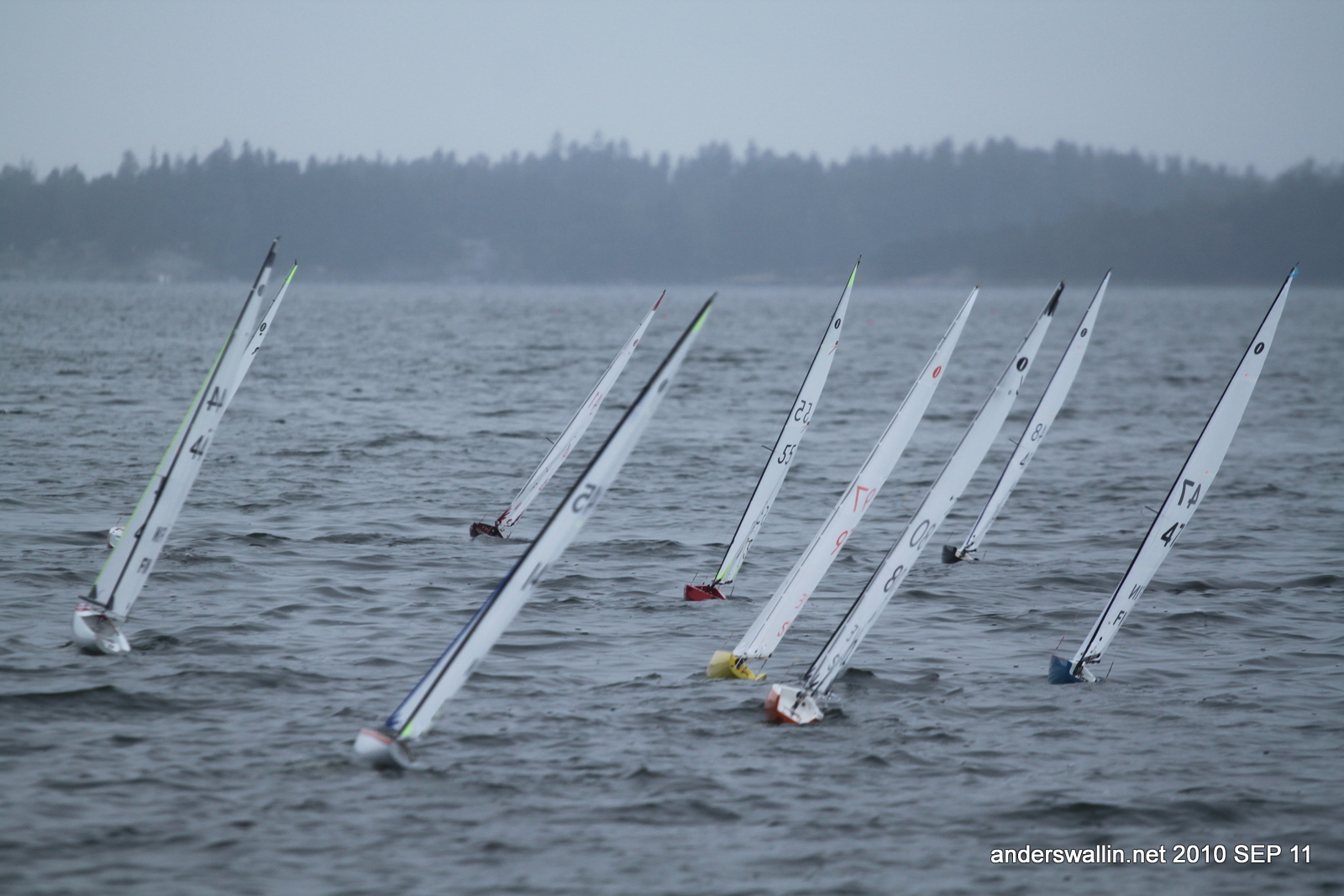
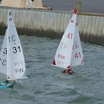
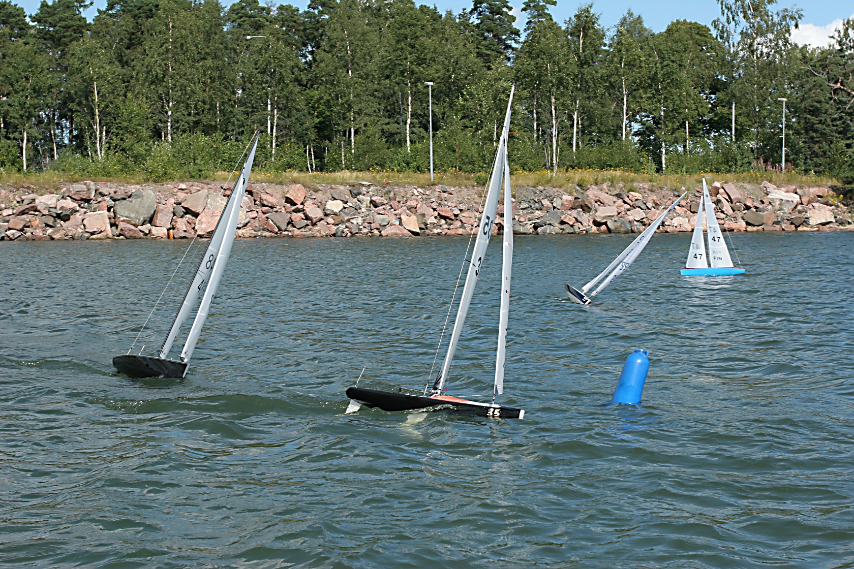
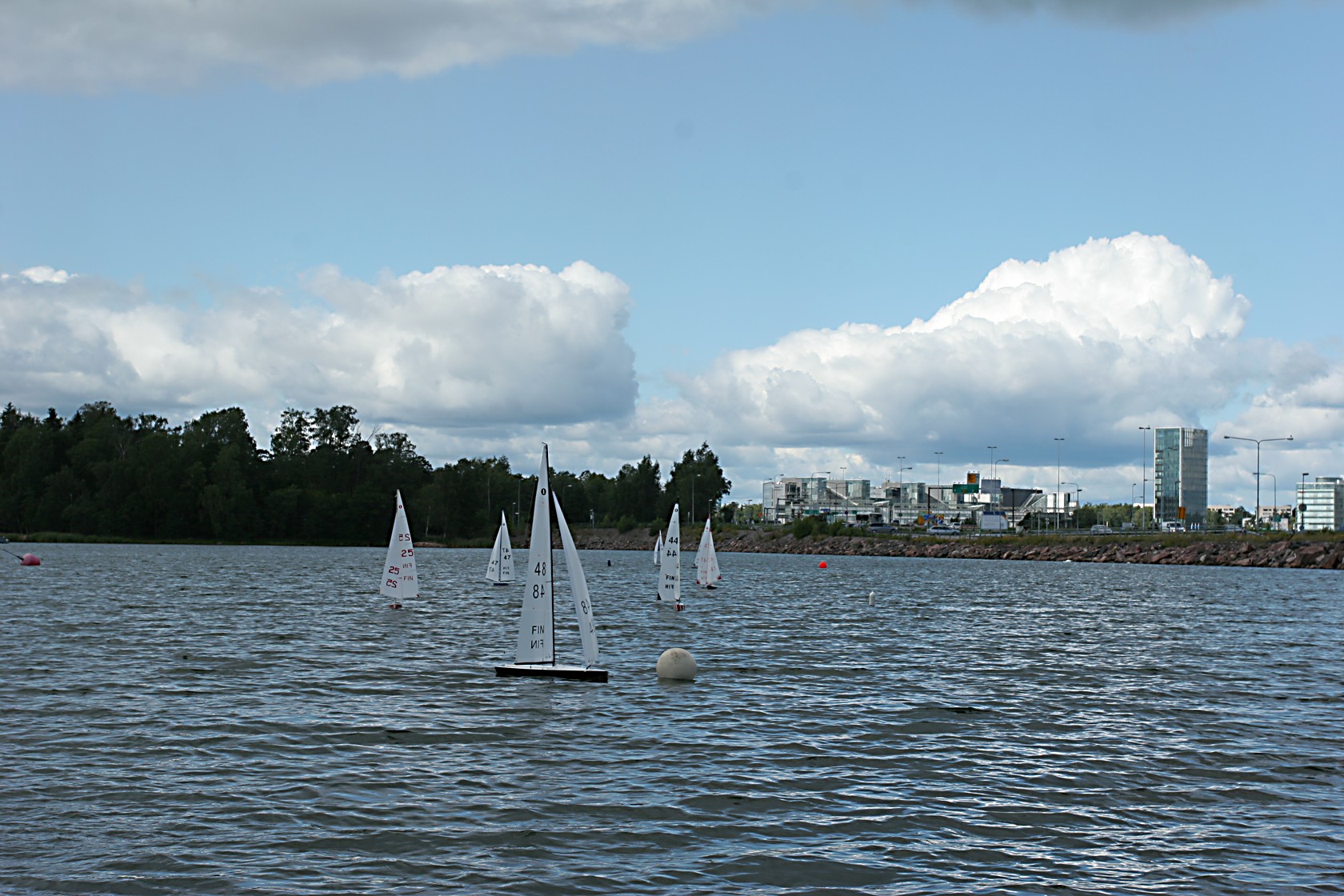
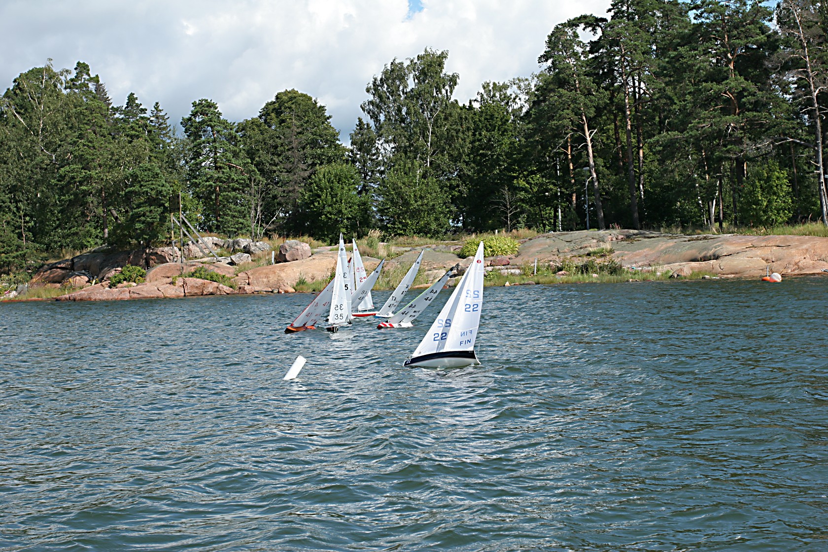
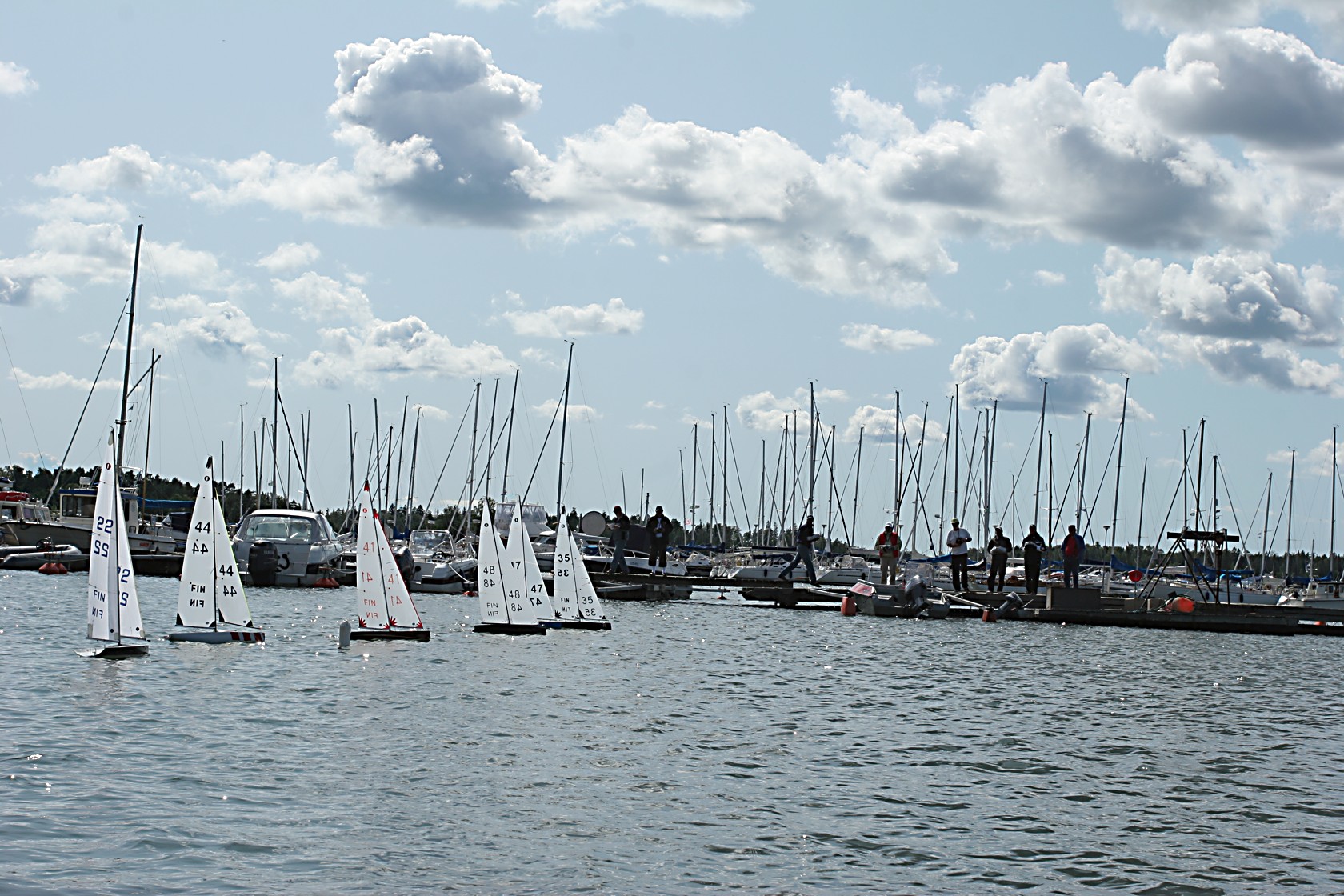
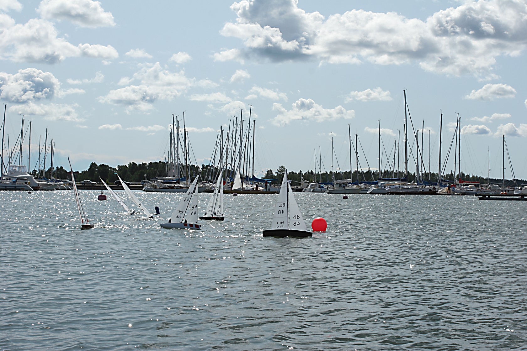
Only 9 skippers (6 FIN, 3 SWE) in this years IOM Nordic Championships, held at NJK Björkholmen, Helsinki.
There are more pictures in picasa: http://picasaweb.google.com/anders.e.e.wallin/2010IOMNordicChampionships#
Preliminary results from day 1: http://www.rc-purjehdus.net/2010/09/2010-iom-nordic-championships-day-1/
I have some incredibly shaky video material shot with the 500D and 70-200 lens which I may or may not upload to youtube later.

Our three-piece hull/deck-moulds for the Pikanto IOM (designed by Graham Bantock) are now ready. The next step is to sand the surface smooth and polish the moulds. We hope to mould a prototype hull before the new year.


The 405cx gps-watch is small and light enough to just tape to the aft-deck of an IOM. Today's event in Tampere had 12 races but I missed a few due to electrical problems. Races 1 and 2 above, and races 7-12 below. It's funny how google-maps and google-earth show permanent winter and ice in Tampere 🙂

The raw-data (tampere_gpsdata.zip) is available in TCX format as well as Google-earth KML format from the garmin connect website.
Anyone have any software or matlab code to extract the instantaneous speed from this data and plot it? Might be useful for further CFD investigations or VPP-programs. Mostly light and shifting no1 rig the whole day. It will be interesting to compare with no2 and no3 rig in a real breeze.
Are there even smaller and lighter GPS-dataloggers? How long before we can have a GPS on every boat and watch playback of the race afterwards at home?

Some details and text on the Computational Fluid Dynamics simulations that mostly Jari has been doing lately. They are done with the open-source software package OpenFOAM, which is of course free to download and use. We run it under Ubuntu, and use fairly affordable 4-core machines with 8 Gb of RAM.
You start with a CAD model of the geometry you want to simulate. Here the hull-shape has been taken from one program, and the sail shape from another sail-design program. They're imported into a third CAD program and joined into the model we want to simulate.
There are (at least!) two issues at this stage: (1) the meshing-tools that follow do not like infinitely thin surfaces, so in order for meshing to run smoothly the sails have to be drawn as having some finite thickness, about 1-2 mm in this case. We can try to reduce this in the future. (2) This is only a CFD simulation, not a fluid-structure interaction simulation. That means the geometry (sails, mast, etc) is not going to move or flex in any way in response to the fluid pressure. So the trim and shape you draw into the sails is going to stay there...
The geometry is exported as STL-files for each surface. Meshing then follows. It's first done with a simple program called blockMesh, and then refined close to any specified surfaces using a program called snappyHexMesh. The resulting mesh looks like this:

And if we zoom in we see the smaller cell-size around the surfaces of the model:

Here's another potential problem with CFD. (3) How do you know what the right mesh-size is? You don't. Decreasing the cell-size obviously leads to a more accurate simulation, but as the size of the mesh goes up the calculation time increases similarly. Some CFD/FEM-packages have adaptive solvers that can increase the mesh-resolution in areas of the simulation where it's most appropriate. I don't know if OpenFOAM has that. One simple approach is to run the same simulation with successively increasing mesh-sizes and see how the end result (e.g. drive force on the model) reaches a plateau, hopefully the correct value.
Then it's time to specify boundary conditions. For a wind-tunnel type of simulation the in-flow velocity on the upwind wall of our simulation-domain is fixed, and the surfaces of the model are specified as no-slip surfaces.
Solving follows. Now you actually have to select the physics model you want to simulate. Well that's easy, in the continuum-limit fluids should behave according to the Navier-Stokes equations. The only problem is that these are nonlinear and difficult to solve. Some people actually do this, but it takes a big big mesh and lot's of computing power. It's called direct numerical simulation. The rest of us with desktop-computers need to solve something simpler than the N-S equations. A lot of different approximations exist, so (4) how do you know which physics model to choose? The Reynolds-averaged N-S equations (RANS) are a popular choice. Our simulations use the simpleFoam solver, which assumes an incompressible fluid, and includes a k-epsilon turbulence model.
OpenFOAM can run the solver on one CPU-core, or the mesh can be split into parts and each part of the mesh run on a separate CPU-core. These simulations usually take around 6-12 hours to complete on a single 2.5 GHz core.
After solving it's time to visualize the results:

OpenFOAM can also integrate the pressure over select parts of the model to obtain the total force on the model. Here we chose a wind-speed and direction for which Lester Gilbert already has some real-world data. The driving and heel-forces seem to roughly agree.
Animations enhance the visual experience:
Add some music and a few camera-angles, and you would think this qualifies as promotional material for any upcoming Americas Cup syndicate...
(To see this in bigger format, click the "YouTube" logo to go their page, and then click "HQ")
That's all for now. If you're a CFD-expert, please be brave and comment below on my open questions (1)-(4) !
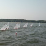
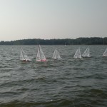
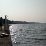
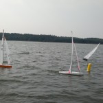
Thanks to Jussi Jaakkola for these images from Saturday's event. It's always nice to sail with the Nr 2 rig, we only get to do that once or twice per season usually.
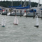
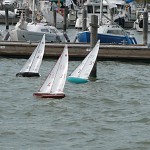
Some pictures from the first day:
And some videos from the second day: (shot with an N95, sorry for the quality...)
Results here.
Does anyone have one of the new Canon or Nikon DSLRs which can record video? With a super-zoom (something like 18-200 mm), is it any good for recording video like this?
Riku and Lasse from the Turku-area IOM-fleet are proud new owners of Jeff Byerley designed Mad Max IOMs. These are the very first boats to come out of Mike Clifton's moulds in the UK. Note black main-boom, I hear it's about 10% faster than the standard aluminum-colored one!