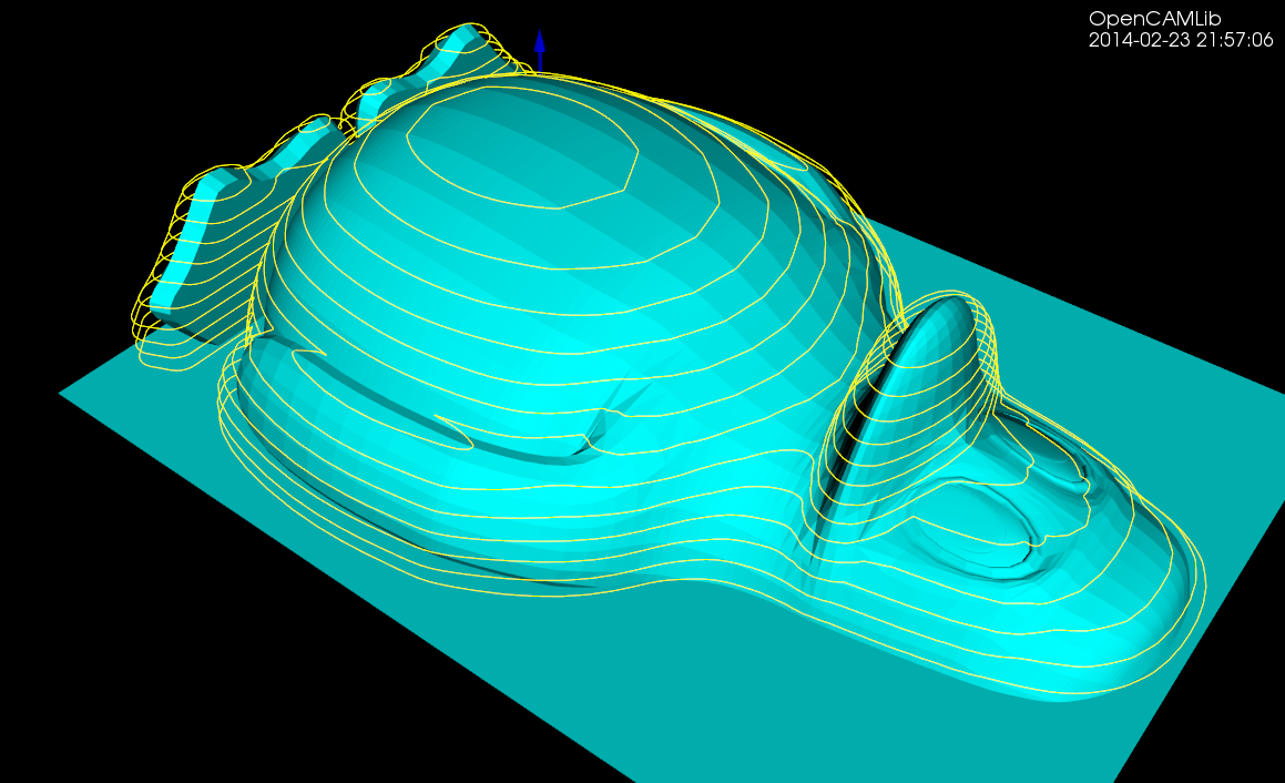
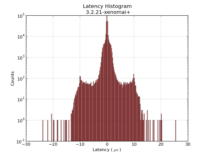
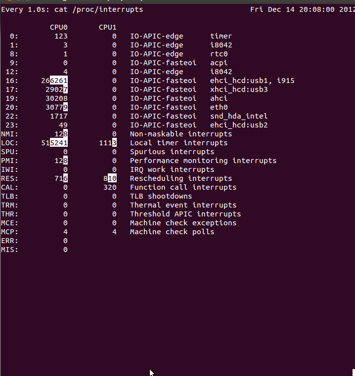
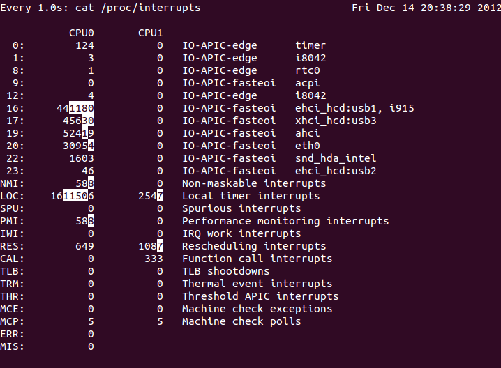
The basic CAM-algorithm called axial tool projection, or drop-cutter, works by dropping down a cutter along the z-axis, at a chosen (x,y) location, until we make contact with the CAD model. Since the CAD model consists of triangles, drop-cutter reduces to testing cutters against the triangle vertices, edges, and facets. The most advanced of the basic cutter shapes is the BullCutter, a.k.a. Toroidal cutter, a.k.a. Filleted endmill. On the other hand the most involved of the triangle-tests is the edge test. We thus conclude that the most complex code by far in drop-cutter is the torus edge test.
The opencamlib code that implements this is spread among a few files:
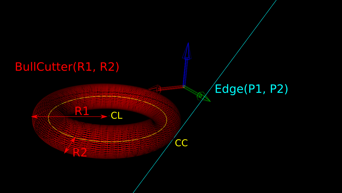
- millingcutter.cpp translates/rotates the geometry into a "canonical" configuration with CL=(0,0), and the P1-P2 edge along the X-axis.
- bullcutter.cpp creates the correct ellipse, calls the ellipse-solver, returns the result
- ellipse.cpp ellipse geometry
- ellipseposition.cpp represents a point along the perimeter of the ellipse
- brent_zero.hpp has a general purpose root-finding algorithm
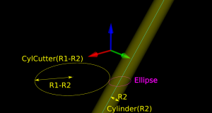
The special cases where we contact the flat bottom of the cutter, or the cylindrical shaft, are easy to deal with. So in the general case where we make contact with the toroid the geometry looks like this:
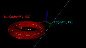
Here we've fixed the XY coordinates of the cutter location (CL) point, and we're using a filleted endmill of radius R1 with a corner radius of R2. In other words R1-R2 is the major radius and R2 is the minor radius of the Torus. The edge we are testing against is defined by two points P1 and P2 (not shown). The location of these points doesn't really matter, as we do the test against an infinite line through the points (at the end we check if CC is inside the P1-P2 edge). The z-coordinate of CL is the unknown we are after, and we also want the cutter contact point (CC).
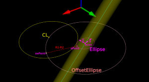
There are many ways to solve this problem, but one is based on the offset ellipse. We first realize that dropping down an R2-minor-radius Torus against a zero-radius thin line is actually equivalent to dropping down a zero-minor-radius Torus (a circle or 'ring' or CylCutter) against a R2-radius edge (the edge expanded to an R2-radius cylinder). If we now move into the 2D XY plane of this circle and slice the R2-radius cylinder we get an ellipse:
The circle and ellipse share a common virtual cutter contact point (VCC). At this point the tangents of both curves match, and since the point lies on the R1-R2 circle its distance to CL is exactly R1-R2. In order to find VCC we choose a point along the perimeter of the ellipse (an ellipse-point or ePoint), find out the normal direction, and go a distance R1-R2 along the normal. We arrive at an offset-ellipse point (oePoint), and if we slide the ePoint around the ellipse, the oePoint traces out an offset ellipse.
Now for the shocking news: an offset-ellipse doesn't have any mathematically convenient representation that helps us solve this!
Instead we must numerically find the best ePoint such that the oePoint coincides with CL. Like so:
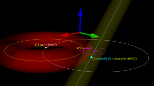
Once we've found the correct ePoint, this locates the ellipse along the edge and the Z-axis - and thus CL and the cutter . If we go back to looking at the Torus it is obvious that the real CC point is now the point on the P1-P2 line that is closest to VCC.
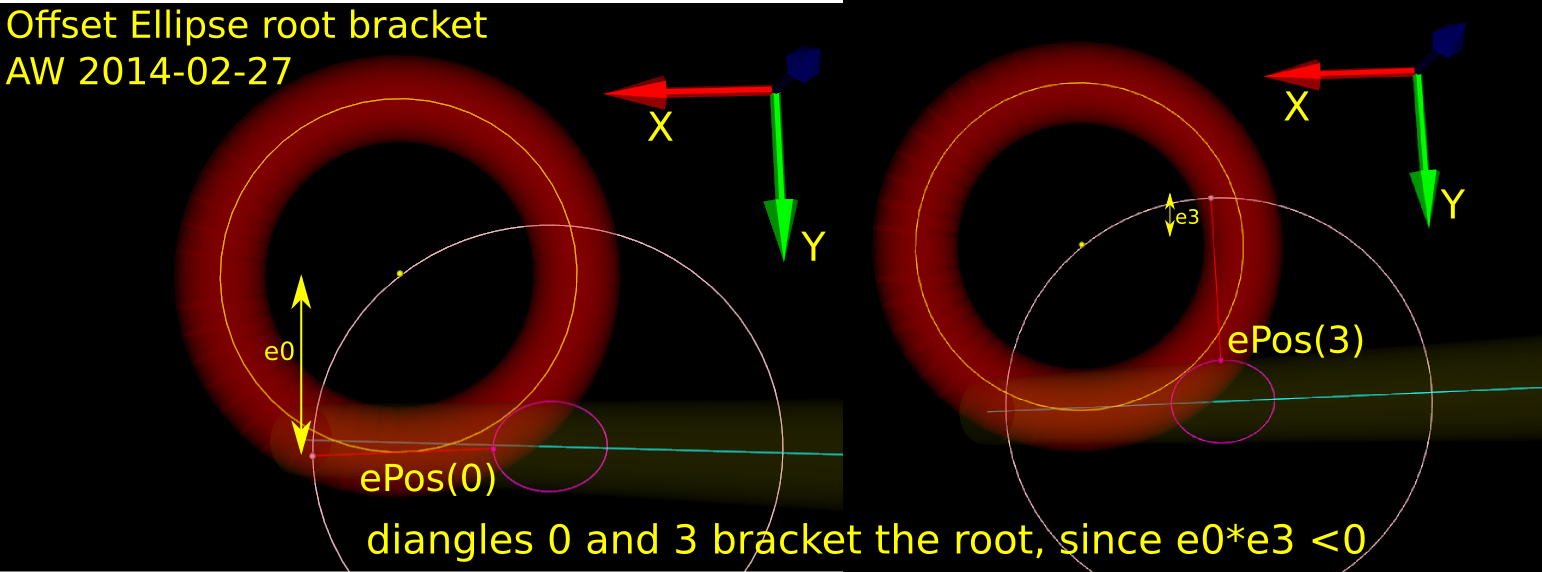
In order to run Brent's root finding algorithm we must first bracket the root. The error we are minimizing is the difference in Y-coordinate between the oePoint and the CL point. It turns out that oePoints calculated for diangles of 0 and 3 bracket the root. Diangle 0 corresponds to the offset normal aligned with the X-axis, and diangle 3 to the offset normal aligned with the Y-axis:

Finally a clarifying drawing in 2D. The ellipse center is constrained to lie on the edge, which is aligned with the X-axis, and thus we know the Y-coordinate of the ellipse center. What we get out of the 2D computation is actually the X-coordinate of the ellipse center. In fact we get two solutions, because there are two ePoints that match our requirement that the oePoint should coincide with CL:
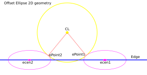
Once the ellipse center is known in the XY plane, we can project onto the Edge and find the Z-coordinate. In drop-cutter we obviously approach everything from above, so between the two potential solutions we choose the one with a higher z-coordinate.
The two ePoint solutions have a geometric meaning. One corresponds to a contact between the Torus and the Edge on the underside of the Torus, while the other solution corresponds to a contact point on the topside of the Torus:
I wonder how this is done in the recently released pycam++?