Temperature PID control

We hooked up the temperature measurement circuit and the PWM-amplifier to EMC today and tested PID-control of the extruder head temperature. The ini, hal, and xml files for this are here: temp_control_pid.tar

It's probably much easier to figure out the connections from the diagram below than to browse the text files. The square wave, which has a frequency proportional to the temperature, comes in on parallel port pin-13, and is connected to an encoder. The encoder has a velocity output which will be equal to the frequency of the square wave in Hz. This frequency is used as the feedback for a PID-component which compares the measured frequency against a set-point which is taken from a pyvcp slider. The pid output is used as an input to a pwm-generator, whose output needs an inverter, since the pwm-amplifier is active-low. The PWM is output on parallel port pin 9.

I wish there was a tool which would draw these HAL/pyVCP diagrams automagically from the source files. There is some work in that direction already: crapahalic and HAL with gschem.

100k sites voronoi diagram

With a bucketing-scheme for nearest-neighbour search in expected time O(1) this voronoi-diagram generation for 100k sites in the [0,1] unit square now runs in 30 s, i.e. it takes about 0.3 ms to insert one point.

Voronoi diagram algorithm

Update: now seems to work for at least 10k generators:

and a zoom-in of the same picture:

One way to compute 2D offsets for toolpath generation is via the voronoi diagram. This video shows the first (somehow) working implementation of my code, which is based on papers by Sugihara and Iri. Their 1992 paper is here: http://dx.doi.org/10.1109/5.163412, then a longer 50-page paper from 1994 here: http://dx.doi.org/10.1142/S0218195994000124, and then there's a more general description of the topology-based approach from 1999 here 10.1007/3-540-46632-0_36, and from 2000 here: http://dx.doi.org/10.1007/s004530010002

The algorithm works by incrementally constructing the diagram while adding the point-generators one by one. This initial configuration is used at the beginning:

The diagram will be correct if new generator points are placed inside the orange circle (this way we avoid edges that extend to infinity). Once about 500 randomly chosen points are added the diagram looks like this:

Because of floating-point errors it gets harder to construct the correct diagram when more and more points are added. My code now crashes at slightly more than 500 generators (due to an assert() that fails, not a segfault - yay!). It boils down to calculating the sign of a 4-by-4 determinant, which due to floating-point error goes wrong at some point. That's why the Sugihara-Iri algorithm is based on strictly preserving the correct topology of the diagram, and in fact they show in their papers that their algorithm doesn't crash when a random error is added to the determinant-calculations, and it even works (in some sense) when the determinant calculation is completely replaced by a random number generator. Their 1992 paper constructs the diagram for one million generators using 32-bit float
numbers, while my naive attempt using double here crashes after 535 points... some work to do still then!

CAM toolpaths tend to be based on CAD-geometry in the form of lines, circular arcs, or spline-curves and such. One way forward is to think of a curve as a lot of closely spaced points along the curve. There are also papers which describe how to extend the algorithm for line and arc generators. See the 1996 paper by Imai. There is FORTRAN code for this by Imai over here (I haven't looked at it or tried compiling it...). Held et al. describe voronoi diagram generation for points and lines in 2001: http://dx.doi.org/10.1016/S0925-7721(01)00003-7 and for points, lines, and arcs in 2009 http://dx.doi.org/10.1016/j.cad.2008.08.004.  This pic from the Held&Huber 2009 paper shows point, line, and arc generators in bold-black, the associated voronoi-diagram as solid lines, and offsets as grey lines.


Held has more pictures here: http://www.cosy.sbg.ac.at/~held/projects/pocket_off/pocket.html

Note how within one voronoi-region the offset is determined by the associated generator (a line, point, or arc). It's very easy to figure out the offset within one region: points and arcs have circular offsets, while lines have line offsets. The complete offset path is a result of connecting the offset from one region with the next region.

Better adaptive waterline

Previously the flat() predicate looked only at the number of intervals contained in a fiber when deciding where to insert new fibers in the adaptive waterline algorithm. Here I've borrowed the same flat() function used in adaptive drop-cutter which computes the angle between subsequent line-segments(yellow), and inserts a new fiber(cyan) if the angle exceeds some pre-set threshold.

This works on the larger Tux model also. However, there's no free lunch: the uniformly sampled waterline (yellow) runs in about 2 s (using OpenMP on a dual-core machine), while the adaptively sampled waterline takes around 30s to compute (no OpenMP).

The difference between the adaptive (red) and the uniformly sampled (yellow) waterlines is really only visible when zooming in on sharp corners or other details. Compare this to adaptive drop-cutter.


EMC2 upgrade

I've upgraded Ubuntu and EMC2 on the Atom 330 machine I have for controlling the lathe. The Atom 330 is a dual-core chip, but with Hyper Threading the OS can see four cores. That's not good for real-time performance, so the first thing I did was turn off HT from the BIOS. Next I did a distribution upgrade to 10.04LTS which downloaded about 1 Gig in an estimated 9 minutes (2Mb/s is OK I guess...). I then used the emc2-install script which installs the real-time kernel and emc2, and finally I edited /boot/grub/menu.lst by adding "isolcpus=1" on the kernel line. This reserves one cpu core for real-time and the other for non-real-time tasks. Without "isolcpus=1" the latency-test jitter values were easily 10k and more with a light load on the machine. With one core dedicated to real-time the jitter numbers start out at around 4k at light load and double to 7-8k under heavy load.

Here are some selected screenshots:

Next stop is getting the X and Z servos moving, as well as the hefty 2 kW spindle servo.

Waterline problem

I was trying to work on a new adaptive waterline feature, but ended up uncovering an old existing problem/bug with waterline. I think it has to be a problem in either building the weave from the fibers, or constructing the planar embedding of the weave.

The yellow waterline should obviously be a smooth loop around the outside of the weave (red/green fibers) and not a zigzag journey back and forth... 🙁

Update: this is better now:

Update2: here's a figure where new fibers (red and green) are inserted adaptively where the shape of the waterline changes most. There's something wrong with building the planar embedding for this weave, so no yellow adaptive waterline path yet...

Update3: some progress at last (fixed a bug in adaptive drop-cutter at the same time):


Adaptive sampling drop-cutter

Inspired by this post on the pycam forum and by this 1993 paper by Luiz Henrique de Figueiredo (or try another version) I did some work with adaptive sampling and drop-cutter today.

The point based CAM approach in drop-cutter, or axial tool-projection, or z-projection machining (whatever you want to call it) is really quite similar to sampling an unknown function. You specify some (x,y) position which you input to the drop-cutter-oracle, which will come back to you with the correct z-coordinate. The tool placed at this (x,y,z) will touch but not gouge the model. Now if we do this at a uniform (x,y) sampling rate we of course face the the usual sampling issues. It's absolutely necessary to sample the signal at a high enough sample-rate not to miss any small details. After that, you can go back and look at all pairs of consecutive points, say (start_cl, stop_cl). You then compute a mid_cl which in the xy-plane lies at the mid-point between start_cl and stop_cl and, call drop-cutter on this new point, and use some "flatness"/collinearity criterion for deciding if mid_cl should be included in the toolpath or not (deFigueiredo lists a few). Now recursively run the same test for (start_cl, mid_cl) and (mid_cl, stop_cl). If there are features in the signal (like 90-degree bends) which will never make the flatness predicate true you have to stop the subdivision/recursion at some maximum sample rate.

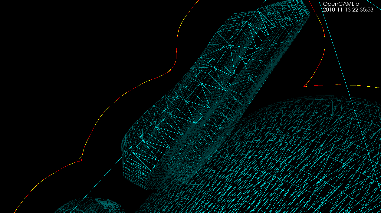
Here the lower point-sequence (toolpath) is uniformly sampled every 0.08 units (this might also be called the step-forward, as opposed to the step-over, in machining lingo). The upper curve (offset for clarity) is the new adaptively sampled toolpath. It has the same minimum step-forward of 0.08 (as seen in the flat areas), but new points are inserted whenever the normalized dot-product between mid_cl-start_cl and stop_cl-mid_cl is below some threshold. That should be roughly the same as saying that the toolpath is subdivided whenever there is enough of a bend in it.

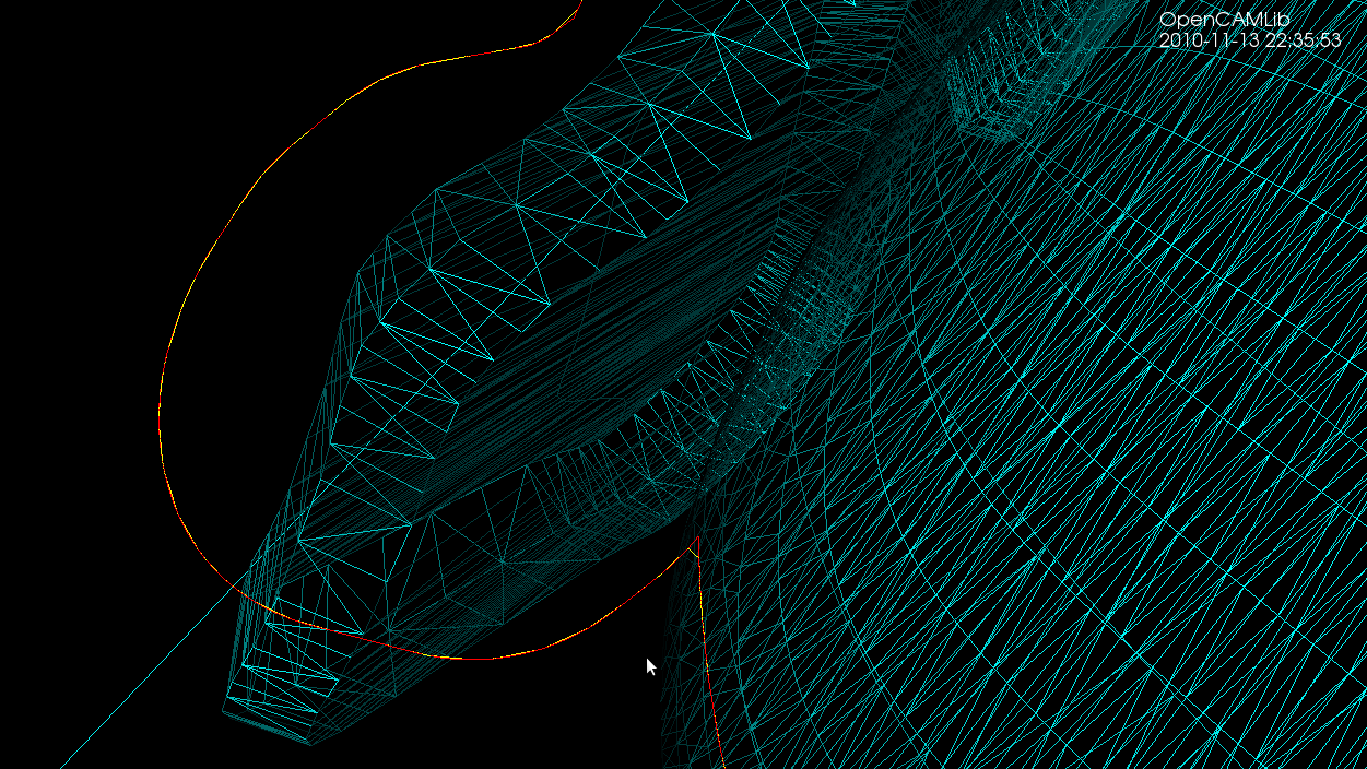
The lower figure shows a zoomed view which shows how the algorithm inserts points densely into sharp corners, until the minimum step-forward (here quite arbitrarily set to 0.0008) is reached.

If the minimum step-forward is set low enough (say 1e-5), and the post-processor rounds off to three decimals of precision when producing g-code, then this adaptive sampling could give the illusion of "perfect" or "correct" drop-cutter toolpaths even at vertical walls.

The script for drawing these pics is: http://code.google.com/p/opencamlib/source/browse/trunk/scripts/pathdropcutter_test_2.py

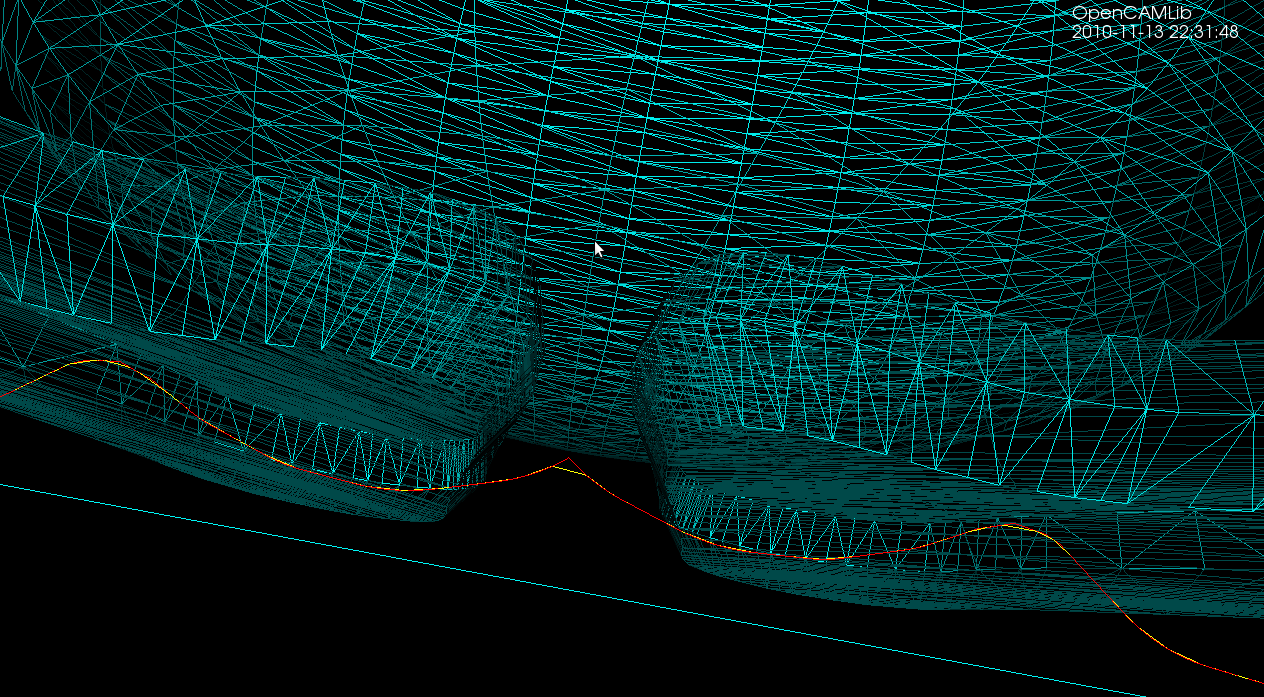
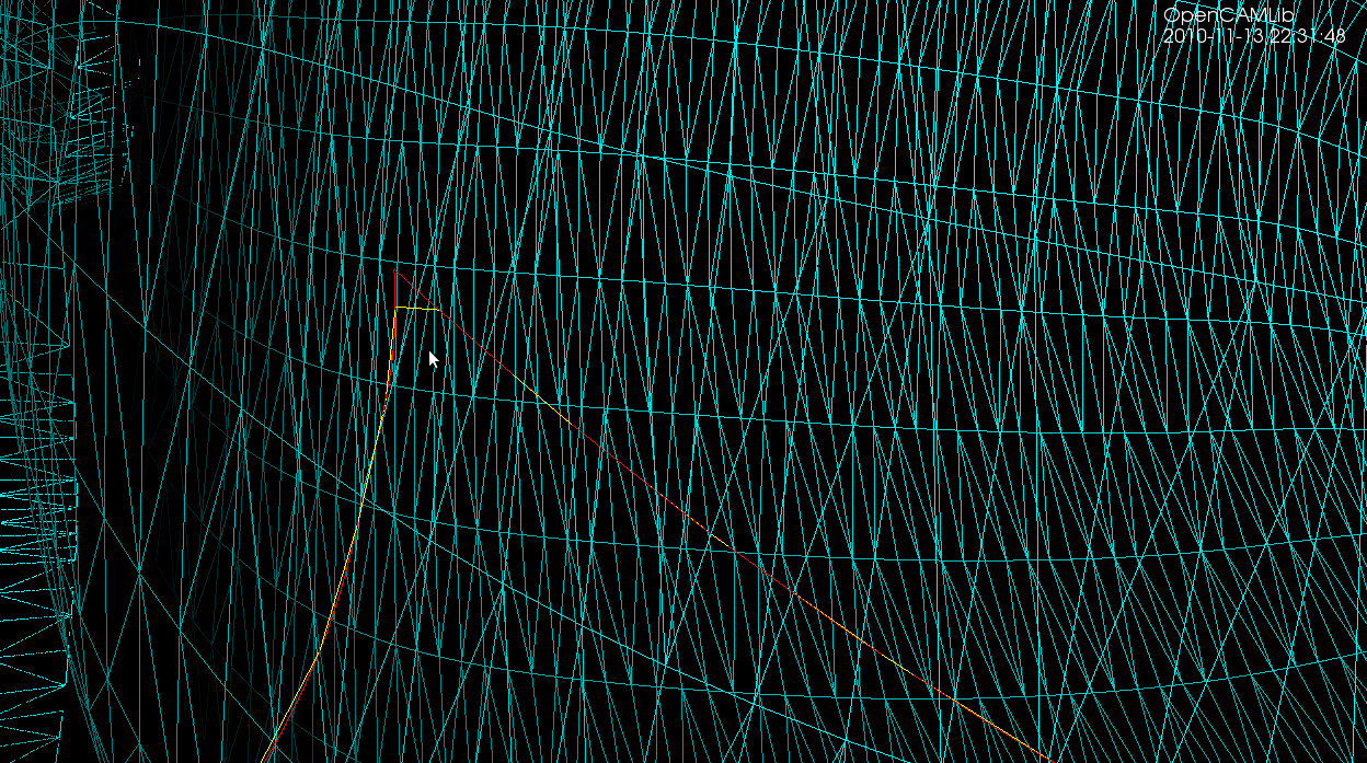
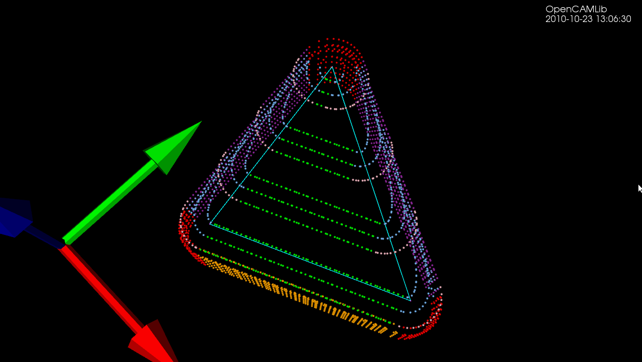
Here is a bigger example where, to exaggerate the issue, the initial sample-rate is very low:

waterline with bullcutter

Update: Here is another example with the CL-points coloured differently. At each z-height the innermost loop is with the ball-cutter, next is the bullcutter, and the outermost loop is calculated for a cylindrical cutter. The points are coloured based on which test (vertex, facet, edge) produced them. Vertex-test points are red. Facet-test points are green. The edge-test is further subdivided into (1) a test for horizontal edges (orange), (2) a test for contact with the cylindrical shaft of the cutter (magenta), and (3) the general edge-push function (light blue for ball/bull, pink for cyl). If/when I get the cone-cutter done the cutter-location algorithms in opencamlib should be complete (at least for the moment...), and I can move on to more interesting high-level algorithms.

three_cutter_waterline

waterline_cutters

This figure shows one of the first times I got the push-cutter/waterline algorithm working for bullcutter (filleted endmill, bull-nose cutter, toroidal cutter, a dear child has many names...).

The thin cyan lines are edges of a triangle. The outer cyan spheres are valid cutter locations (CL-points) for a cylindrical endmill. The innermost yellow CL-points are for a spherical (or ball-nose) endmill. Between these two point-sets the new development is the magenta points, which are CL-points for a bull-nose cutter.

The algorithm works by pushing the cutter at a specified Z-height along either the X-axis or the Y-axis into contact with the triangle. There are three sub-functions for handling the case where the cutter makes contact with a vertex, the triangle facet, and an edge. The edge-contact case is the non-trivial (read "hard") one. The approach I am using is based on the offset-ellipse, courtesy of the freesteel blog. Pushing a toroid into contact with an edge/line is equivalent to pushing the cylindrical "core" of the bullcutter into contact with an edge that has been 'inflated' to a cylinder with a radius equal to the bullcutter corner radius. Slicing this cylinder/tube with a z-plane gives us an ellipse, and the sought cutter-location lies on the offset of this ellipse. I should make some diagrams and post longer/better explanation later (I wonder if anyone reads these 🙂 ).

The bullcutter is important not only in itself, but also because it is the offset of a cylindrical cutter. When we want to do z-terrace roughing with a cylindrical cutter, and specify a stock-to-leave value, we do it by calculating the toolpath with cylcutter->offsetCutter() which is a bullcutter, and then actually machining with the cylindrical cutter. That will achieve the desired stock to leave (to be removed later by a finish operation).