opencamlib – Page 3 – anderswallin.net

Waterline toolpaths, part 2

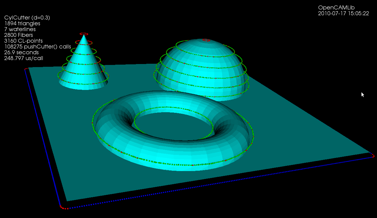
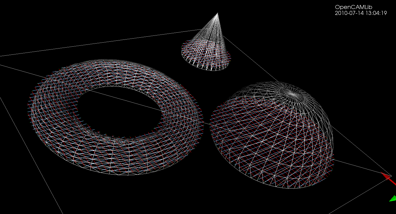
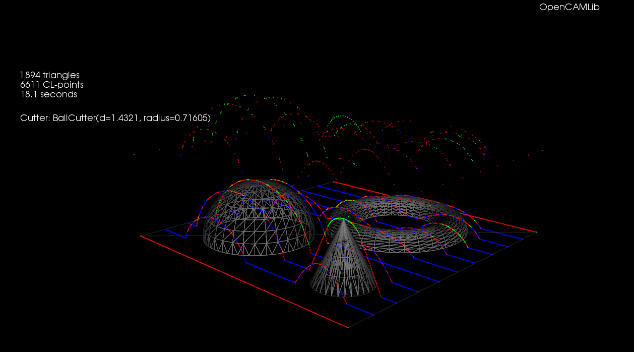
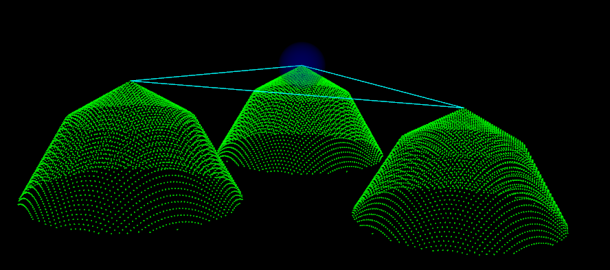
After the proof-of-principle waterline experiments two days ago I've modified the KD-tree search so that triangles overlapping with the cutter can be searched for in the XZ and YZ planes (in addition to the XY-plane, which was needed for drop-cutter). This dramatically reduces the number of triangles which go through the pushCutter function and makes it possible to run some tests on small to medium STL files.

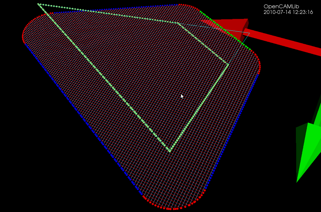
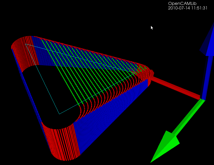
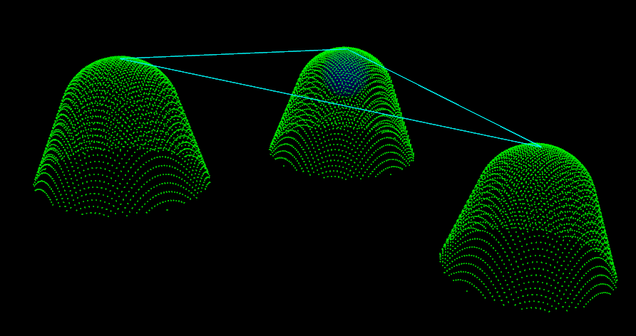
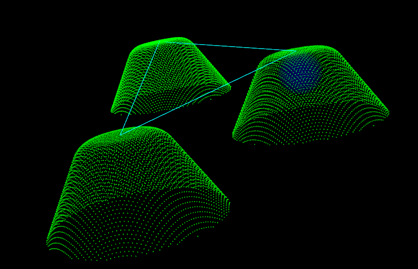
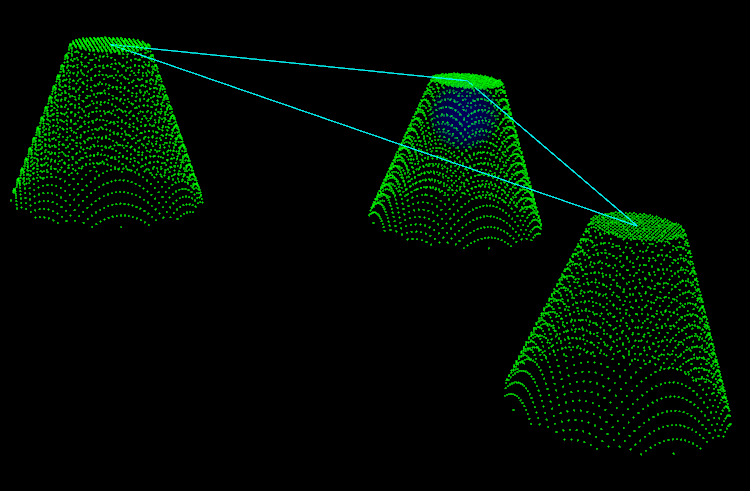
Currently all the CL-points come out of the algorithm in an undefined almost random order. I'm just plotting them all and they are closely spaced, so it looks like a path, but the algorithm has no idea in which order the CL-points should be visited. Before these waterlines are of any use a second algorithm is required which inspects the weave and (a) comes up with the number of "loops" or "rings" (what should we name these?) at each waterline and (b) sorts the CL-points in each loop into the right order. The upstream user of these waterline loops can then decide in which order to visit the waterlines at each z-height, and within one waterline in which order to visit the loops. Any CL-point in a loop is as good as any other, so the upstream user can also choose where to start/stop the toolpath around the loop.

My idea for this is to turn the weave in to a graph and use the Boost Graph Library which has a function for returning the number of connected components (part (a) above), and then perhaps the All-pairs shortest path algorithm to find adjacent CL-points (part (b) above). Any other ideas?

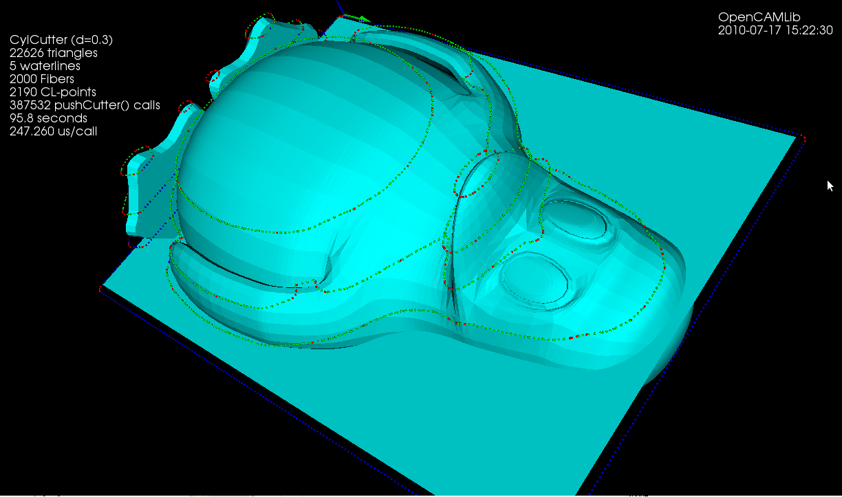
Here's the obligatory Tux example, where it took 96 seconds to generate five waterlines.

Waterline toolpath experiment

The logical next step from drop-cutter ("axial tool projection" or "z-projection machining") is to instead push the cutter sideways("radial tool projection") against the model and get waterline (or "z-slice") paths. In addition to waterline finish-paths these paths can be used in roughing where they define pockets for 2D machining/clearing of stock. The general purpose tool-location function would be a non-axial tool projection, but I'm not going there unless someone sends me a state of the art 5-axis VMC as a present!

Push-cutter is different from drop-cutter, because in drop-cutter for 3-axis machining there is always only one right answer. There's one z-height where the cutter is positioned as low as possible, but doesn't interfere with the model. In drop-cutter positioning the tool above this z-height is OK, but dropping it further down is an illegal move which causes overcutting.

In push-cutter we push the cutter along a line (called a "fiber") in the xy-plane, and search for CL-points where the cutter touches a triangle, together with illegal points or stretches/intervals along the fiber where the cutter interferes. There are going to be many of these points and intervals, so the fiber needs to keep track of everything using a list of interfering intervals (the endpoints of the intervals are valid CL-points).
Similarly to drop-cutter, where a path is sampled along points in the (x, y) plane, we now need to build up our waterline-path by inserting closely spaced fibers in the x-direction and the y-direction. Eventually the CL-points start to form a continuous waterline, if we hook up the points into a list in the correct order. The x- and y-fibers form a grid (or mesh/weave), a kind of graph, which can be used to figure out the correct ordering of the CL-points (not implemented yet, see BGL).

This picture shows the original triangle (thin cyan lines), X-fibers (red lines), Y-fibers (blue lines), and the endpoints of the fibers, which are CL-points (colored by which element of the triangle they are hitting: red=vertex, green=facet, blue=edge). The light-green points are CC-points, i.e. points where the cutter makes contact with the triangle. This initial experiment uses a cylindrical cutter, and I expect the spherical cutter to follow soon, while the toroid will be more difficult...

This picture does not show the fibers/weave, only CL-points, calculated at many different z-heights.

If the low-level functions are written right these ideas extend easily from the one-triangle test and debugging case to the practically more important and interesting many-triangle case: (note how now the weave-graph has three disconnected components)

Coming to an open-source CAM-system near you this summer/fall...

Cutsim Tux

Octree-based cutting simulation

Here's an initial test of octree-based cutting simulation:

If you turn up the resolution to eleven, where it starts to be useful and not so grainy, the calculation of the tool-swept volume, which we subtract from the stock at each move, becomes too slow.
See also octree operations.

Download a short clip with a depth=10 tree: OUTPUT (it's also on youtube, but a 2s clip on youtube doesn't work very well: http://www.youtube.com/watch?v=G0RYS9FcqR0)

some screenshots:

Line filter for opencamlib

When generating toolpaths with drop-cutter ("axial tool-projection", if you like fancy words) the path ends up being composed of lots of short linear segments. It makes sense to filter this list of points and take out any middle points that lie on a straight line between neighboring points. Here's a first attempt at such a line-filter.

The lower points is the raw output from drop cutter, while the filtered points are offset vertically for clarity. There are 6611 CL-points in the raw data, but only 401 CL-points after filtering.

The next step is to come up with an arc-filter which detects circular arcs in the list of CL-points. All CNC-machines have G2/3 circular arc motion in the principal planes (xy, xz, yz). Then the number of moves will go even further down from 401 points.

This is just something to live with, having chosen the triangulated model approach to CAM. First we have pure and exact shapes in CAD which get tessellated into zillions of tiny triangles, from these we generate a sampled toolpath consisting of lots and lots of points, and finally we filter to get back those "pure" "exact" and "nice" line-segments and arcs.

The relevant part of the code looks like this. It might be a bit prettier to use the remove_if STL algorithm? Also, there's no check that p1 actually lies between p0 and p2.

    typedef std::list<clpoint>::iterator cl_itr;
    cl_itr p0 = clpoints.begin();
    cl_itr p1 = clpoints.begin();
    p1++;
    cl_itr p2 = p1;
    p2++;
    for(  ; p2 != clpoints.end(); ) {
        Point p = p1->closestPoint(*p0, *p2);
        if ( (p- *p1).norm() < tol )  { // p1 is to be removed
            p1 = clpoints.erase(p1);
            p2++;
        } else {
            p0++;
            p1++;
            p2++;
        }
    }

full code here.

Composite cutters for ocl

People who, unlike me, actually know something about programming often talk about design patterns. One common idea is to compose objects out of other objects.

I was able to add four new APT-tool like cutter classes to ocl with about 5-lines of code for each cutter (sans the bugfixing, taking much longer, that also took place simultaneously 🙂 ).

These show CL-points resulting from the vertexDrop() function, which results in a shape that looks like the cutter, but inverted.

Other combinations of the basic shapes (cylinder, sphere, torus, cone) are fairly easy to add now also if someone actually needs them.

Drop-Cutter examples

I've experimented with using OpenMP to calculate drop-cutter toolpaths on a quad-core machine. These now run reasonably fast. There are obvious lurking bugs with BallCutter and BullCutter still...

Code is here: code.google.com/p/opencamlib/ (if you know C++, computational geometry, and cnc-machining, or are willing to learn, this project needs your help!)

Cutting down the octree

If you number the octants in an octree using a 1982 scheme called Gargantini-code, and store the codes for only the black nodes in the tree in a list then that's called a linear octree.

For quadtrees, there is a 1985 paper by Bauer with an algorithm for computing set-operations (intersection, union, difference) between two trees. Ten years later Jiang corrected a few mistakes and extended this algorithm to octrees. Neither paper is free of misprints, but by looking at both I seem to have arrived at set-operations which work.

Pushing lists with 10 000 or more elements back and forth between C++ and python is not very fast, and I'm now rendering each node (a cube) in a tree as a separate Cube-object in VTK, which isn't very efficient. The video shows depth 6 trees at the end, and here's a screen-capture of a depth 7 tree:

This could be useful for making a cutting-simulator used for both verifying CAM-algorithms in opencamlib, and G-code produced by other programs. It's probably possible to hook into the EMC2interpreter and have it drive the tool in the simulation.

Toroidal drop-cutter

A one-triangle test of drop-cutter for toroidal tools (a.k.a. filleted-endmills, or bull-nose).

The blue points are contacts with the facet, and the green points are contacts with the vertices. These are easy.

The edges-contacts (red-points) are a bit more involved, and are done with the offset-ellipse solver presented earlier here(the initial geometry) and here(offset-ellipse construction) and here(convergence of the solver) and here(toroid-line intesection animation).

Octree in python

Recursion and 'divide-and-conquer' must be two of the greatest ideas ever in computer science.

Threw together some code in python today for building an octree, given a function isInside() which the tree-builder evaluates to see if a node is inside or outside of the object. Nodes completely outside the interesting volume(here a sphere, for simplicity) are rendered grey. Nodes completely inside the object are coloured, green for low tree-depth, and red for high. Where the algorithm can't decide if the node is inside or outside we subdivide (until we reach a decision, or the maximum tree depth).

In the end our sphere-approximation looks something like this:

These tests were done with a maximum tree depth of 6 or 7. If we imagine we want a 100 mm long part represented with 0.01 mm precision we will need about depth 14, or a subdivision into 16384 parts. That's impractical to render right now, but seems doable. In terms of memory-use, the octree is much better than a voxel-representation where space is uniformly subdivided into tiny voxels. The graph below shows how the number of nodes grows with tree-depth in the actual octree, versus a voxel-model (i.e. a complete octree). For large tree-depths there are orders-of-magnitude differences, and the octree only uses a number of nodes roughly proportional to the surface area of the part.

Now, the next trick is to implement union (addition) and difference (subtraction) operations for octrees. Then you represent your stock material with one octree, and the tool-swept-volume of your machining operation with another octree -> lo and behold we have a cutting-simulator!