Tag: opencamlib
Delaunay Triangulation
The dual of the Voronoi diagram is the Delaunay triangulation. Here I've modified my earlier VD code to also output the dual (shown in red). If this can be developed further to do constrained Delaunay triangulations (arbitrary pockets with islands) then it will be useful for cutter-location surfaces in opencamlib.
The regular grid is, in the words of the GTS website, "a much more difficult test than it looks".
Adaptive sampling drop-cutter
Inspired by this post on the pycam forum and by this 1993 paper by Luiz Henrique de Figueiredo (or try another version) I did some work with adaptive sampling and drop-cutter today.
The point based CAM approach in drop-cutter, or axial tool-projection, or z-projection machining (whatever you want to call it) is really quite similar to sampling an unknown function. You specify some (x,y) position which you input to the drop-cutter-oracle, which will come back to you with the correct z-coordinate. The tool placed at this (x,y,z) will touch but not gouge the model. Now if we do this at a uniform (x,y) sampling rate we of course face the the usual sampling issues. It's absolutely necessary to sample the signal at a high enough sample-rate not to miss any small details. After that, you can go back and look at all pairs of consecutive points, say (start_cl, stop_cl). You then compute a mid_cl which in the xy-plane lies at the mid-point between start_cl and stop_cl and, call drop-cutter on this new point, and use some "flatness"/collinearity criterion for deciding if mid_cl should be included in the toolpath or not (deFigueiredo lists a few). Now recursively run the same test for (start_cl, mid_cl) and (mid_cl, stop_cl). If there are features in the signal (like 90-degree bends) which will never make the flatness predicate true you have to stop the subdivision/recursion at some maximum sample rate.

Here the lower point-sequence (toolpath) is uniformly sampled every 0.08 units (this might also be called the step-forward, as opposed to the step-over, in machining lingo). The upper curve (offset for clarity) is the new adaptively sampled toolpath. It has the same minimum step-forward of 0.08 (as seen in the flat areas), but new points are inserted whenever the normalized dot-product between mid_cl-start_cl and stop_cl-mid_cl is below some threshold. That should be roughly the same as saying that the toolpath is subdivided whenever there is enough of a bend in it.
The lower figure shows a zoomed view which shows how the algorithm inserts points densely into sharp corners, until the minimum step-forward (here quite arbitrarily set to 0.0008) is reached.

If the minimum step-forward is set low enough (say 1e-5), and the post-processor rounds off to three decimals of precision when producing g-code, then this adaptive sampling could give the illusion of "perfect" or "correct" drop-cutter toolpaths even at vertical walls.
The script for drawing these pics is: http://code.google.com/p/opencamlib/source/browse/trunk/scripts/pathdropcutter_test_2.py
Here is a bigger example where, to exaggerate the issue, the initial sample-rate is very low:
waterline with bullcutter
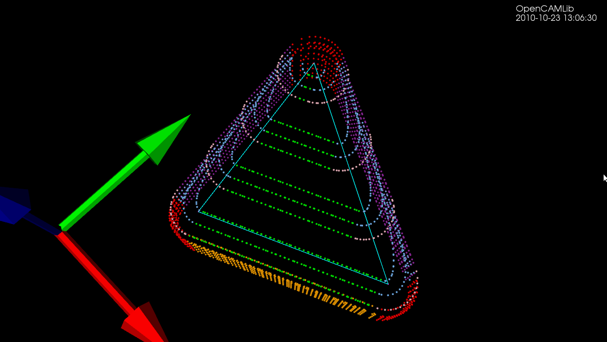
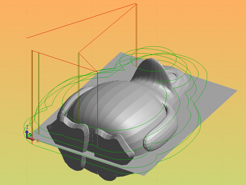
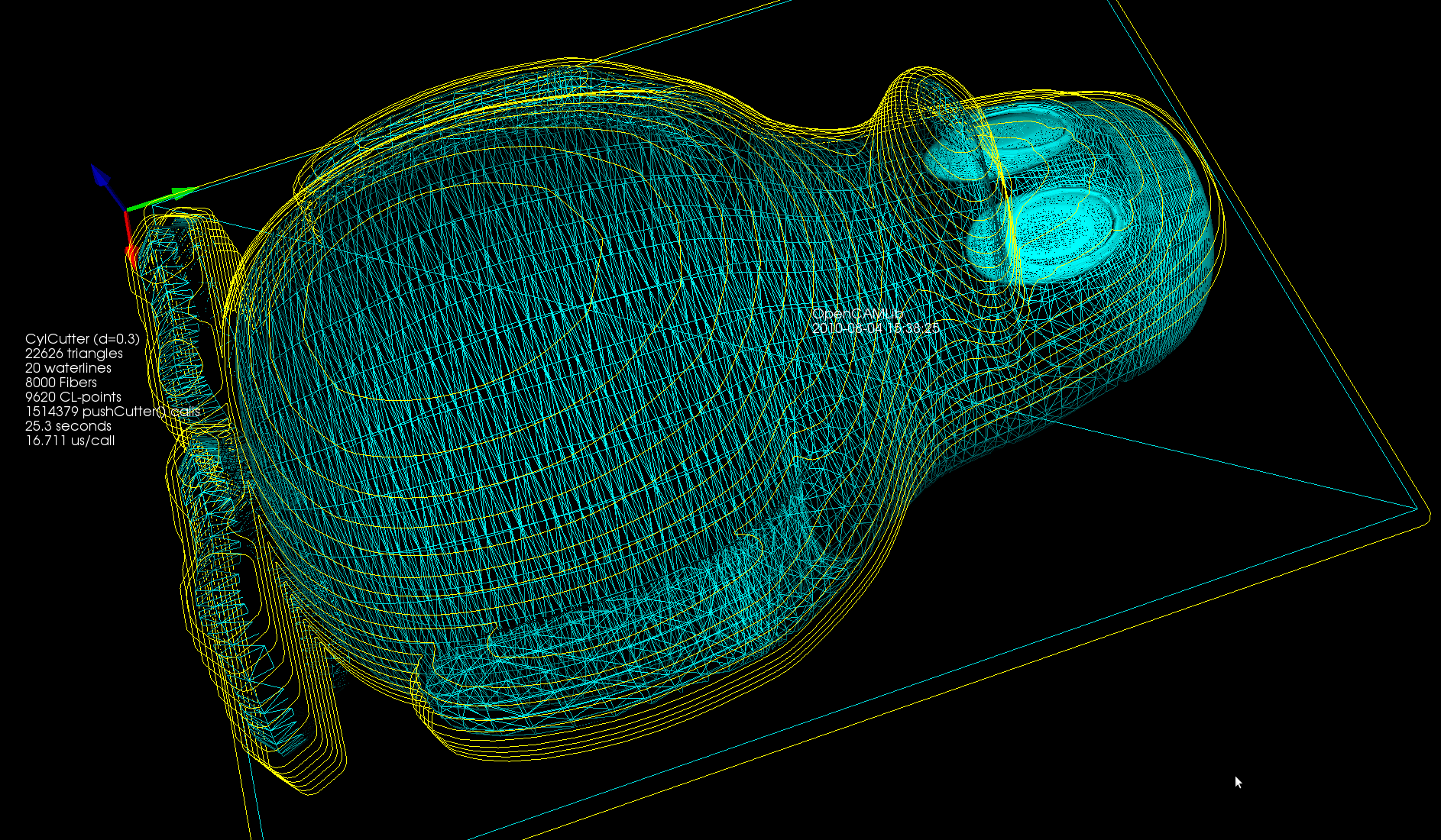
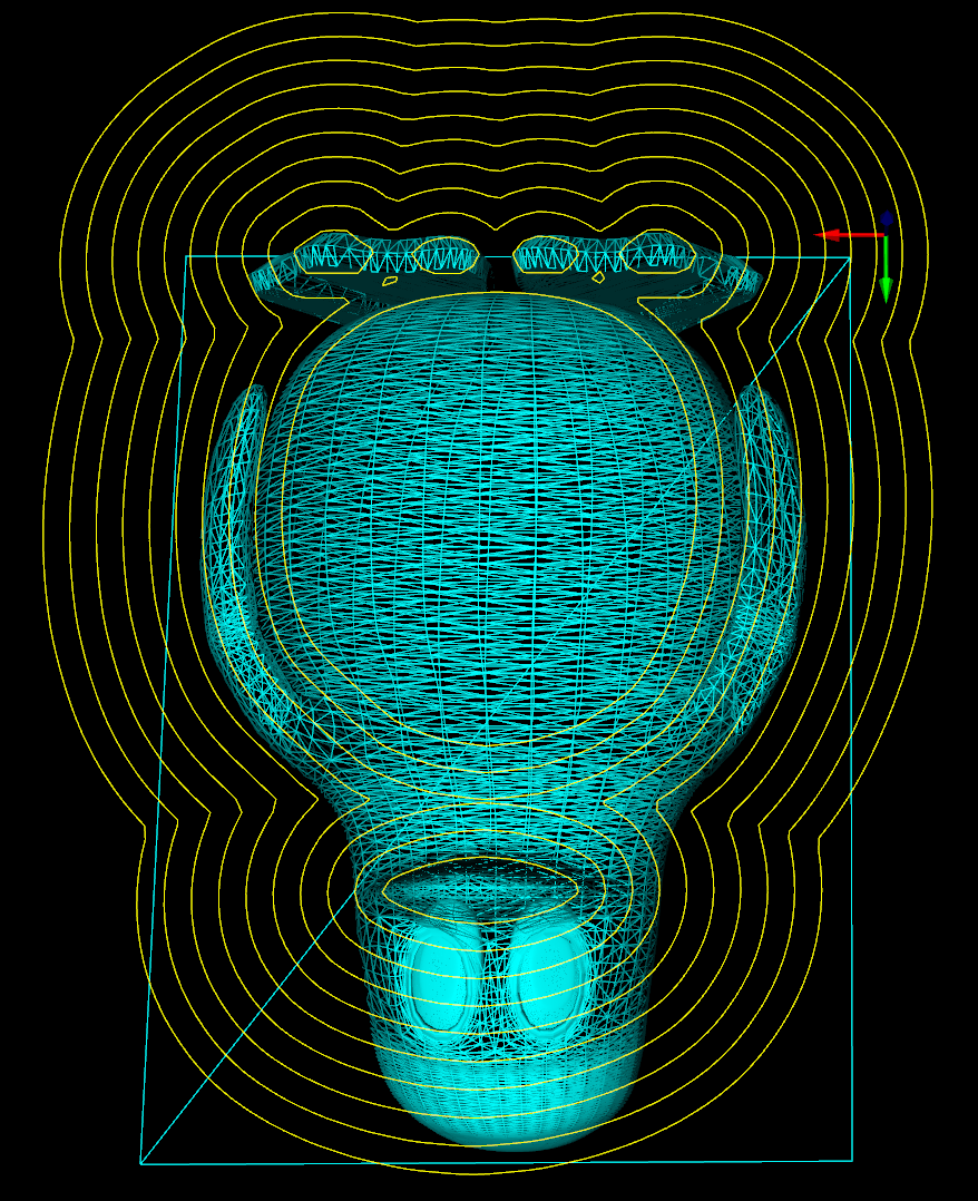
Update: Here is another example with the CL-points coloured differently. At each z-height the innermost loop is with the ball-cutter, next is the bullcutter, and the outermost loop is calculated for a cylindrical cutter. The points are coloured based on which test (vertex, facet, edge) produced them. Vertex-test points are red. Facet-test points are green. The edge-test is further subdivided into (1) a test for horizontal edges (orange), (2) a test for contact with the cylindrical shaft of the cutter (magenta), and (3) the general edge-push function (light blue for ball/bull, pink for cyl). If/when I get the cone-cutter done the cutter-location algorithms in opencamlib should be complete (at least for the moment...), and I can move on to more interesting high-level algorithms.
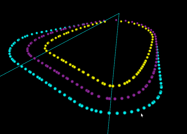
This figure shows one of the first times I got the push-cutter/waterline algorithm working for bullcutter (filleted endmill, bull-nose cutter, toroidal cutter, a dear child has many names...).
The thin cyan lines are edges of a triangle. The outer cyan spheres are valid cutter locations (CL-points) for a cylindrical endmill. The innermost yellow CL-points are for a spherical (or ball-nose) endmill. Between these two point-sets the new development is the magenta points, which are CL-points for a bull-nose cutter.
The algorithm works by pushing the cutter at a specified Z-height along either the X-axis or the Y-axis into contact with the triangle. There are three sub-functions for handling the case where the cutter makes contact with a vertex, the triangle facet, and an edge. The edge-contact case is the non-trivial (read "hard") one. The approach I am using is based on the offset-ellipse, courtesy of the freesteel blog. Pushing a toroid into contact with an edge/line is equivalent to pushing the cylindrical "core" of the bullcutter into contact with an edge that has been 'inflated' to a cylinder with a radius equal to the bullcutter corner radius. Slicing this cylinder/tube with a z-plane gives us an ellipse, and the sought cutter-location lies on the offset of this ellipse. I should make some diagrams and post longer/better explanation later (I wonder if anyone reads these 🙂 ).
The bullcutter is important not only in itself, but also because it is the offset of a cylindrical cutter. When we want to do z-terrace roughing with a cylindrical cutter, and specify a stock-to-leave value, we do it by calculating the toolpath with cylcutter->offsetCutter() which is a bullcutter, and then actually machining with the cylindrical cutter. That will achieve the desired stock to leave (to be removed later by a finish operation).
OpenCAMLib from HeeksCNC
I've tried using opencamlib through heekscnc. With a few minor modifications to the ocl_funcs.py script I got it working. Although ocl prints some debug information and a progress bar to the console when run standalone, I couldn't find that window in heekscnc. Even with this small example there are obvious issues with memory management (sometimes 8 Gb wasn't enough!) on either the heekscnc or ocl-side of things (or both!).
On Ubuntu 10.04LTS getting all the bits and pieces, compiling them and installing them was a breeze thanks to this install script. However the GUI feels very "sticky" with the mouse cursor not really going where I want it to go, and the keyboard focus being in surprising places when I want to edit properties. It must be possible to make a GUI that feels good to use with wxgtk, right?
I think currently the inputs and outputs of these two operations, "ZigZag" and "Waterline", are defined in at least three places: ocl itself, the python script ocl_funcs.py, and in the heekscnc c++ GUI code that displays the menus and buttons. Something like introspection or reflection or naked objects would be needed so that a GUI can query the libraries that are present on what operations they offer, what input they need, and what output they produce. If I get my head around some generic-enough GUI ideas I might try writing something myself also. Most probably based on Qt and VTK. In any case the cutting-simulation needs to be driven from a C++ GUI, for performance, I think.
Octree animation
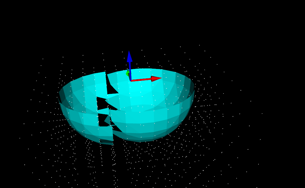
Update: this figure shows the numbering of vertices(red), edges(green), and faces(blue). The arrows show the direction of the X-(red), Y-(green), and Z-axes(blue).

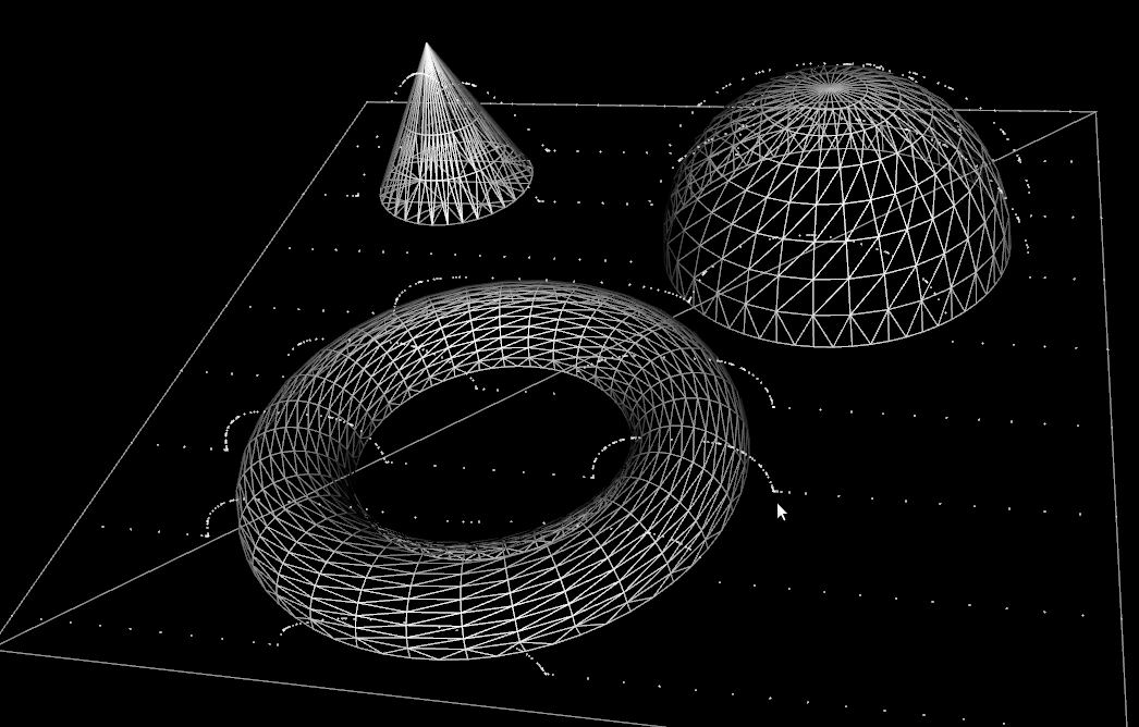
Here the sides of the cube are not generated with Marching-Cubes, they are just extracted directly from the octree. Nodes are subdivided whenever the signed distance-field of the cutter indicates that the surface is contained within the node, i.e. the distance-field evaluates to both positive and negative at the eight fourvertices of a node. This apparently leads to transient holes in the surface when the cutter is just about to enter a coarse node which hasn't been subdivided very far yet. It should be possible to adjust the subdivision criterion so that the octree 'anticipates' the cutter slightly and subdivides ahead of the actual cutter surface.
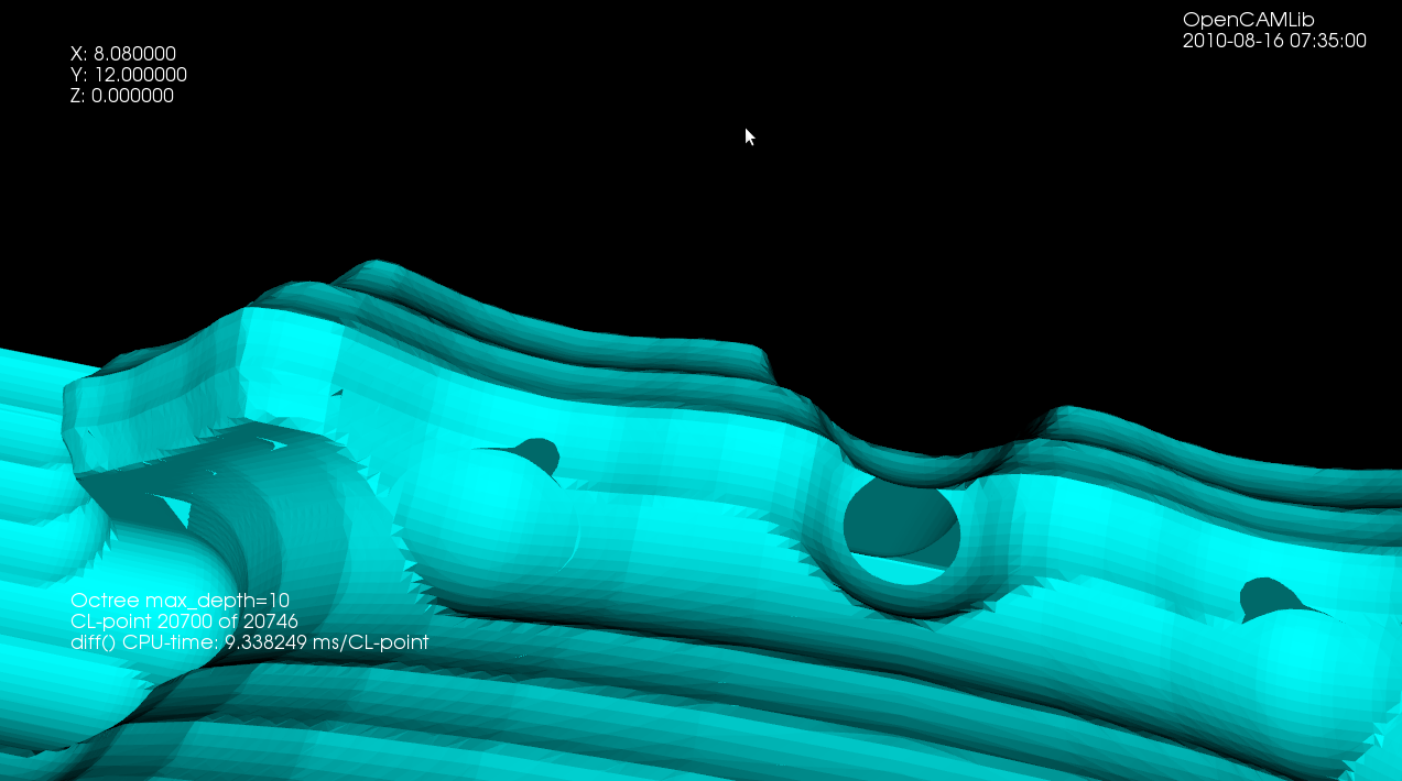
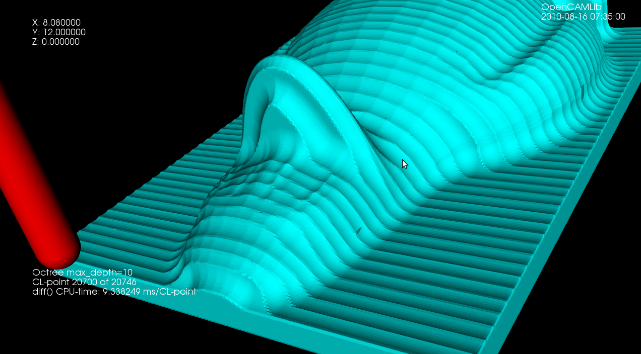
Cutsim progress
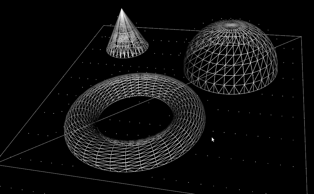
The speed of the new cutting-simulation code makes it possible to run it at a higher resolution than before. That makes the surfaces look smooth and nice. Alas, some problems still remain with holes in the fabric of reality mystically appearing and disappearing .
There is an edge-flipping paper by Kobbelt et al. from 2001 which improves the jagged/aliased look of sharp edges.
Update: Kobbelt provides a LGPLv2 licensed sample-implementation of the algorithm here: http://www-i8.informatik.rwth-aachen.de/index.php?id=17
Octree with Marching Cubes
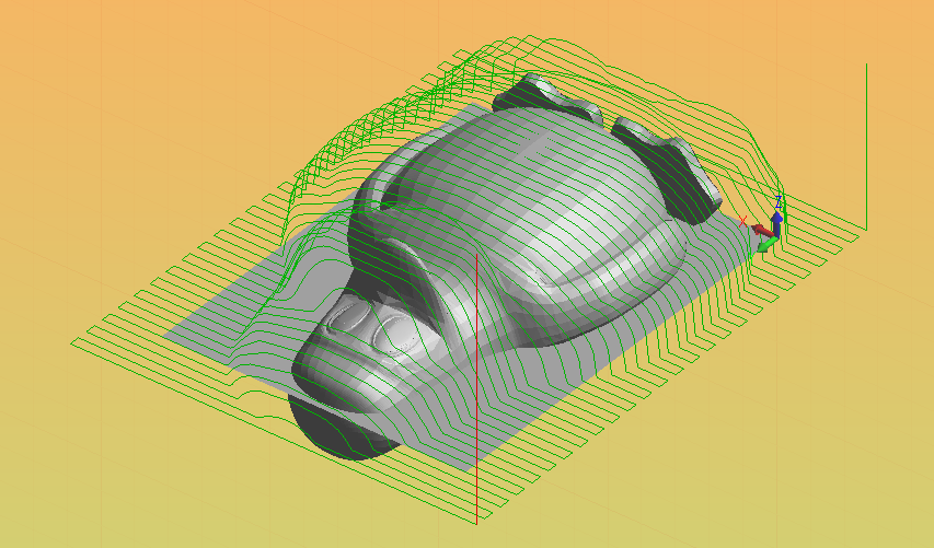
Update 3: this leads slowly towards a better and faster cutting simulation. Here's an example with Tux:

Update2: this looks slightly better now (a ball translated in a few steps towards the right). Image and c++ code by fellow OCLer Jiang from China.

Update: in a cutting simulation the stock is updated by removing voxels which fall inside the cutter. Here I'm trying it with a spherical shape positioned at (0,0), and then moved slightly along the X-axis. The white dots are corners of octree nodes, and the cyan triangles are produced by marching cubes. It works quite well, but on the border between the two cutter instances the distance-field is somehow wrong, and marching-cubes doesn't come up with the right triangles, leaving gaps instead.
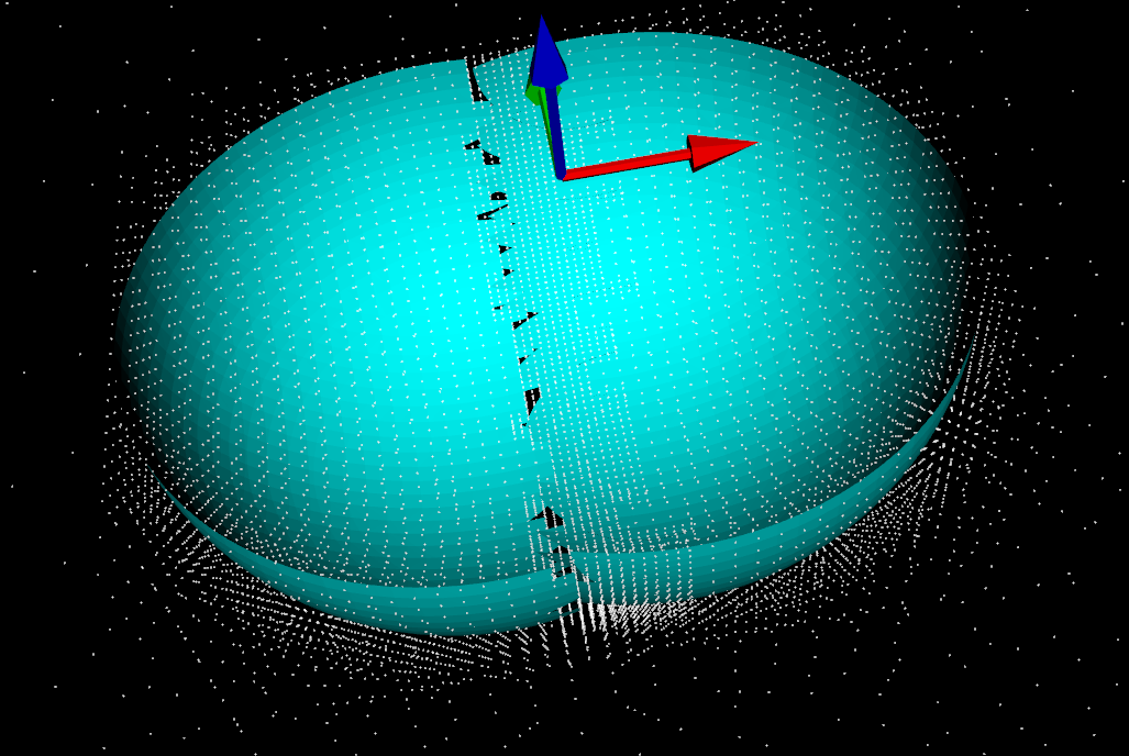
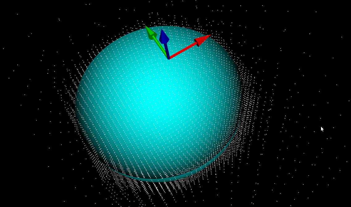
Earlier I was building an octree volume-representation of a shape using a simple bool isInside(Point p) predicate function to determine which cubes are in and which are out. If instead a distance-function double distance(Point p) which is negative inside the volume, zero exactly on the surface, and positive outside, is used, then the Marching Cubes algorithm (this is a better explanation, someone should make the wikipedia page as good!) can be used to triangulate the octree. This leads to much more visually pleasing results at reasonable maximum tree-depths.
The same Hong-Tzong Yau of Taiwan who wrote a very reasonable drop-cutter paper in 2004 has more recently come out with a 2009 paper on cutting simulation using an octree and Marching Cubes.
The weave point-order problem
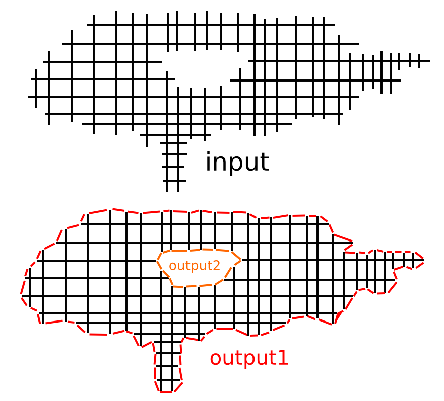
When creating waterlines or 2D offsets using a "sampling" or "CL-point based" approach the result is a grid or weave such as that shown in black above. The black lines can in principle be unevenly spaced, and don't necessarily have to be aligned with the X/Y-axis. The desired output of the operation is shown in red/orage, i.e. a loop around/inside this weave/grid, which connects all the "loose ends" of the graph.
My first approach was to start at any CL-vertex and do a breadth_first_search from there to find the closest neighboring vertices. If there are many candidates equally close you then need to decide where to jump forward, and do the next breadth_first_search. This is not very efficient, since breadth_first_search runs a lot of times (you could stop the search at a depth or 5-6 to make it faster).
The other idea I had was some kind of 'surface tension', or edge removal/relaxation where you would start at an arbitrary point deep inside the black portion of the graph and work your way to the outside as far as possible to find the output. I haven't implemented this so I'm not sure if it will work.
What's the best/fastest way of finding the output? Comments ?!
Update: I am now solving this by first creating a planar embedding of the graph and then running planar_face_traversal with a visitor that records in which order the CL-points were visited. The initial results look good:
Waterline toolpaths, part 3
I've written a function that looks at the weave and produces a boost adjacency-list graph of it. The graph can then be split up into separate disconnected components using connected_components. To illustrate this, the second highest waterline in the picture below has six disconnected components: around the beak, belly, and toes(4). When we know we are dealing with one connected component we pick a starting point at random. I'm then using breadth_first_search from this starting point to find the distance, along the graph, from this starting CL-point to all other CL-points. We choose the point with the minimum distance (along the graph) as the next point. Sometimes many points have the same distance from the source vertex and another way of choosing between them is required (I'm now picking the one which is closest in 2D distance to the source, but this may not be correct). We then mark the newly found CL-point "done", and proceed with another breadth_first_search with this vertex as the source. That means that the graph-search runs N times if we have N CL-points, which is not very efficient...
So, compared to previously, we now have for each waterline a list-of-lists where each sub-list is a loop, or an ordered list of CL-points. The yellow lines connect adjacent CL-points.
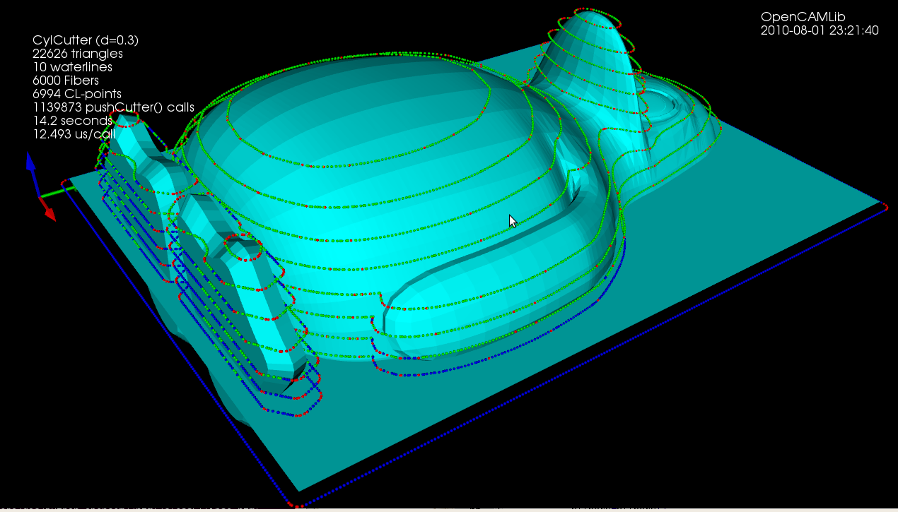
There's still a donut-case, where one connected component of the weave produces more than one loop, which the code doesn't handle correctly.