anderswallin.net

Photon-correlation test with modulated LED

Further testing of the time-stamping hardware. The idea was to generate a weak beam of light with an intensity modulation at 1-12 MHz, count and time-stamp the photons, and see if the modulation can be measured with a correlation histogram.

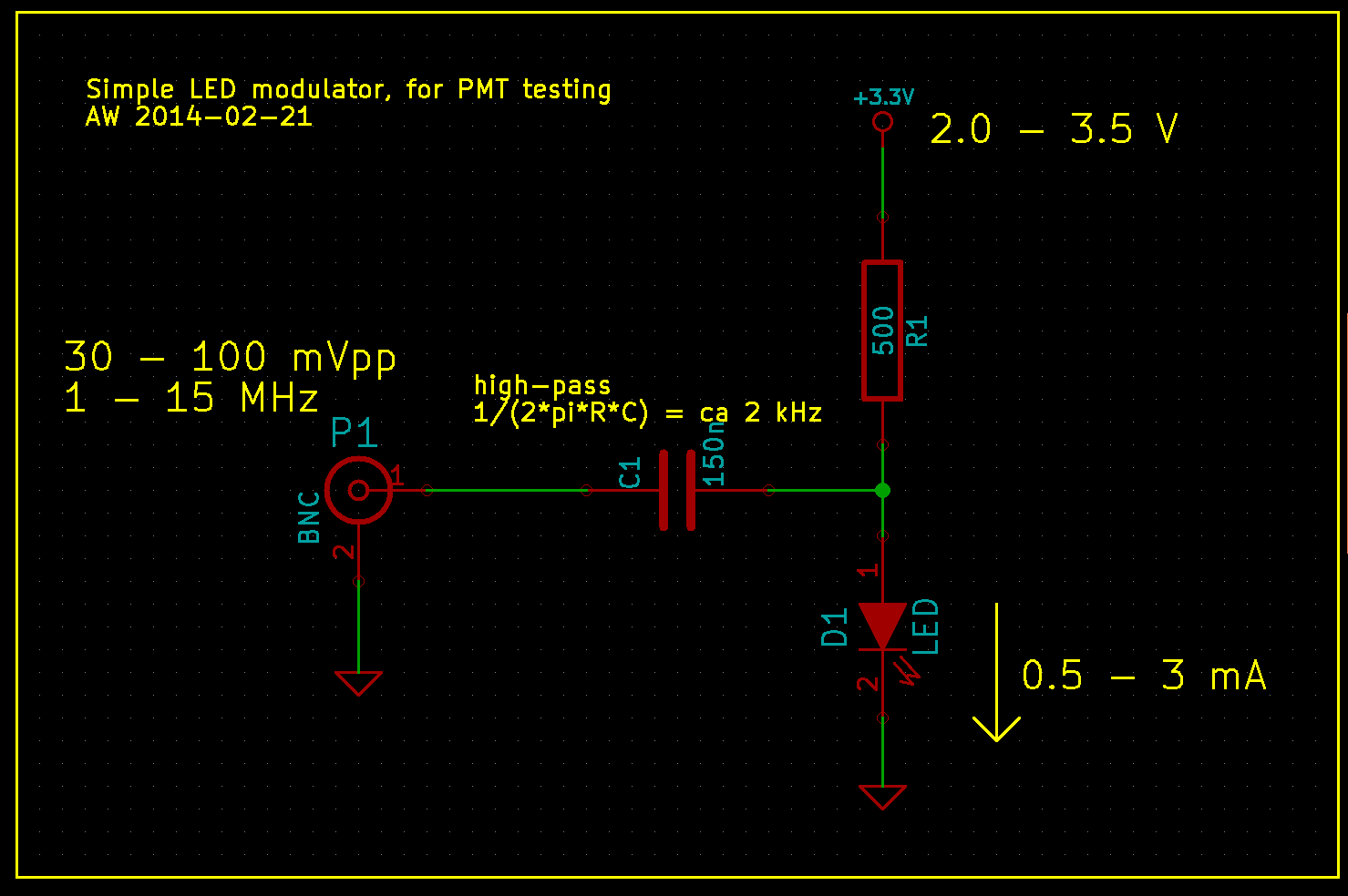
To generate a stream of photons intensity modulated at a frequency f_mod I used this simple LED circuit driven by an adjustable DC power-supply and a signal generator. I didn't test the bandwidth of the circuit and LED, but it seems to work well for this test at least up to 12 MHz.

If we are given such a stream of photons, with an average rate of say 10 kphotons/s, how do we detect that the modulation at MHz frequencies is there? Note that the average rate of photons is much much smaller than the modulation frequency. If we receive photons at 10 kcounts/s there is on average 1000 cycles of modulation between each photon-event, when f_mod=10 MHz.

One way is to count the photons with a photon-counter, and time-stamp each photon. We should now on average see more/less photons every 1/f_mod seconds. So if we histogram all time stamps modulo 1/f_mod, we should get a sine-shaped histogram. This assumes that the signal generator creating f_mod and our time-stamping hardware share a common time-base.

This works quite nicely!

At the start of the video we see only the dark counts of the PMT. A DC voltage is then applied to the LED and the histogram rises up, but remains flat. When the modulation is applied we immediately see a sine-shape of the histogram. If we adjust the the frequency, phase, or amplitude of the modulation we see a corresponding change in the histogram.

The video first has testing at f_mod=1 MHz, with a histogram modulo 1/f_mod = 1000 ns, and later with f_mod=12 MHz and the histogram modulo 83333 ps. The later part of the video also has a least-squares sin() fit to the data.

This technique is very sensitive to mismatch between the applied frequency f_mod, and the histogram mod-time 1/f_mod. I first wanted to try this at 12 MHz, so I set the histogram mod-time to 83333 ps - and saw no sine-histogram at all! This was because I had rounded 1/f_mod to the nearest picosecond, and 1/83333 ps is actually 12 000 048 Hz - not 12 MHz!
At 12 MHz a deviation of 48 Hz is a few ppm in fractional frequency, and I later tested that changing f_mod by a fraction of ca 1e-8 makes the histogram slowly wander to the left or right. Any larger deviation and the correlation is lost.
All of this is similar to a lock-in technique, so the same principles should apply.

White Rabbit Fine-Delay time-stamp testing

I'm testing the White Rabbit Fine-Delay FMC. It has an ACAM TDC-GXP time-to-digital converter that time-stamps the leading edge of an input trigger signal with ~30 ps resolution.

Recent work by Alessandro Rubini introduced a raw_tdc=1 driver mode which on my computer is able to collect time-stamps at a maximum rate of ca 150 kHz. Each time-stamp is 24-bytes, so this corresponds to a data-stream of roughly 4 Mb/s.

The video shows two graphs that update in real-time on the machine that collects time-stamps. The first is simply a (reciprocal) frequency counter where we count how many time-stamps arrive within a certain gate/window.

The second part of the video shows a modulo(tau) histogram where we bin time-stamps modulo tau into a histogram. The histogram was calculated for tau=100 us and an input frequency of 1 kHz was used. This results in the central peak in the histogram. I then slightly increased the frequency to 1.000010 kHz which makes the peak wander to the right. The peak on the right was produced by again tuning the input frequency to exactly 1 kHz. Similarly a lower input frequency of 999.970 Hz makes the peak wander to the left, and the peak around 20us was produced after tuning back to 1 kHz.

This hardware/software combination will be useful for collecting statistics and correlations in any experiments where a pulse type detector is used to measure something - provided the pulse-rate is below 150 kHz or so.

Pulse Stretcher - v1

A first try at this pulse stretcher circuit based on the LT1711 comparator. I need it for stretching a short 10ns pulse from a PMT.

The idea is to use the output latch of the LT1711. Once the output goes high, the combination C4 R4 keeps the latch pin (and thus the output) high for a time R*C. The Schottky diode is there to prevent the latch pin from swinging to far negative once the output goes low.

The PCB is made to fit into a BNC-BNC enclosure such as the ones from Pomona.

Messing up the pin-order of voltage regulators is becoming a habit! Note how the regulator is mounted the wrong way round compared to the PCB design - because I had the pin order wrong in my schematic.

I used a Keithley 50 MHz function generator to generate a 20ns long input pulse (the shortest possible from the Keithley) and the pulse-stretcher outputs a ca 483 ns output pulse. The prototype used a 1 nF capacitor with a 500 Ohm resistor which gives a nominal time-constant of 500 ns. The output pulse duration is far from constant and varies quite a bit from pulse to pulse.

This verifies that the propagation delay of the LT1711 in this circuit is within specifications, ca 4.5 ns. In addition to the comparator there is also maybe 70 mm of BNC-connectors, wires, and PCB-traces in the signal path, but that would add only ~350 ps to the propagation delay (assuming 2e8 m/s signal velocity).

One problem with this design is that it is sensitive to the load impedance connected to the output. With a 1 MOhm setting on the oscilloscope the pulse-length is correct, but switching to a 50 Ohm load impedance allows the capacitor to discharge significantly through the load impedance.

Version 2 of this circuit should thus add an output buffer (fast, low-jitter!) that can drive both 1 MOhm and 50 Ohm loads. An adjustable trigger level for the -Input of the LT1711 comparator could also be useful.

ZeromMQ REQuest/REPly pattern

More zeromq testing. See also PUB/SUB.

This pattern is for a reply&request situation where one machine asks for data from another machine. The pattern enforces an exchange of messages like this:

REQuester always first sends, then receives.

REPlyer always first receives, then sends.

Requester

import zmq
import time
 
# request data from this server:port
server = "192.168.3.38"
port = 6000
 
context = zmq.Context()
socket = context.socket(zmq.REQ)
socket.connect ("tcp://%s:%s" % (server,port) )
 
while True:
    tstamp = time.time()
    msg = "%f" % tstamp # just send a timestamp
    # REQuester: TX first, then RX
    socket.send(msg)        # TX first
    rep = socket.recv() # RX second
    done = time.time()
    oneway = float(rep)-tstamp
    twoway = done - tstamp
    print "REQuest ",msg
    print "REPly   %s one-way=%.0f us two-way= %.0f us" % ( rep, 1e6*oneway,1e6*twoway )
    time.sleep(1)
 
# typical output:
# REQuest  1392043172.864768
# REPly   1392043172.865097 one-way=329 us two-way= 1053 us
# REQuest  1392043173.866911
# REPly   1392043173.867331 one-way=420 us two-way= 1179 us
# REQuest  1392043174.869177
# REPly   1392043174.869572 one-way=395 us two-way= 1144 us

The one-way delay here assumes we have machines with synchronized clocks. This might be true to within 1ms or so if both machines are close to the same NTP server.

The two-way delay should be more accurate, since we subtract two time-stamps that both come from the REQuesters system clock. Much better performance can probably be achieved by switching to C or C++.

Replyer:

import zmq
import time
 
port = 6000
context = zmq.Context()
socket = context.socket(zmq.REP)
# reply to anyone who asks on this port
socket.bind("tcp://*:%s" % port) 
 
print "waiting.."
while True:
    #  Wait for next request from client
    message = socket.recv() # RX first
    print "Received REQuest: ", message
    tstamp = time.time()
    sendmsg = "%f" % tstamp # send back a time-stamp
    print "REPlying: ",sendmsg
    socket.send(sendmsg) # TX second
 
# typical output:
# Received REQuest:  1392043244.206799
# REPlying:  1392043244.207214
# Received REQuest:  1392043245.209014
# REPlying:  1392043245.209458
# Received REQuest:  1392043246.211170
# REPlying:  1392043246.211567

ZeroMQ PUB/SUB pattern

I'm playing with zeromq for simple network communication/control. For a nice introduction with diagrams see Nicholas Piel's post "ZeroMQ an introduction"

Here is the PUBlish/SUBscribe patter, which usually consist of one Publisher and one or many Subscribers.

Publisher:

import zmq
from random import choice
import time
 
context = zmq.Context()
socket = context.socket(zmq.PUB)
socket.bind("tcp://*:6000") # publish to anyone listening on port 6000
 
countries = ['netherlands','brazil','germany','portugal']
events = ['yellow card', 'red card', 'goal', 'corner', 'foul']
 
while True:
    msg = choice( countries ) +" "+ choice( events )
    print "PUB-> " ,msg
    socket.send( msg ) # PUBlisher only sends messages
    time.sleep(2)
 
# output:
# PUB-> netherlands yellow card
# PUB-> netherlands red card
# PUB-> portugal corner

And here is the Subscriber:

import zmq
 
context = zmq.Context()
socket = context.socket(zmq.SUB)
# specific server:port to subscribe to
socket.connect("tcp://192.168.3.35:6000") 
# subscription filter, "" means subscribe to everything
socket.setsockopt(zmq.SUBSCRIBE, "") 
 
print "waiting.."
while True:
	msg = socket.recv() # SUBscriber only receives messages
	print "SUB -> %s" % msg
 
# typical output:
# waiting..
# SUB -> portugal corner
# SUB -> portugal foul
# SUB -> portugal foul

allantools

Python code for calculating Allan deviation and related statistics: https://github.com/aewallin/allantools

Sample output:

Cheat-sheet (see http://en.wikipedia.org/wiki/Colors_of_noise).

Phase PSD	Frequency PSD	ADEV
1/f^4, "Black?"	1/f^2, Brownian, random walk	sqrt(tau)
1/f^3 ?, "Black?"	1/f Pink	constant
1/f^2, Brownian, random walk	f^0, White	1/sqrt(tau)
f^0, White	f^2 Violet	1/tau

Phase PSD is frequency dependence of the the power-spectral-density of the phase noise.
Frequency PSD is the frequency dependence of the power-spectral-density of the frequency noise.
ADEV is the tau-dependence of the Allan deviation.

These can get confusing! Please comment below if I made an error!

White Rabbit DIO vs. FDELAY PPS output test

I ran a test to compare the quality of PPS outputs from a DIO (used as GM) and an FDELAY (used as slave) White Rabbit SPEC/FMC combinations. Here is the phase data measured with a Time-interval-counter. The nice clean traces are derived from a H-maser. We then lock a BVA (internally 2x multiplied to 10MHz) to this PPS signal. The GM node is locked to this 10MHz signal.

The average of each trace was removed, and the traces are offset for clarity.

The Allan deviations look like this. Both the DIO and FDELAY PPS outputs have allan deviations about 5x worse than the BVA used as input clock for the GM.

AD9912 DDS Test

Update: it turns out the PLL filter components were not connected at all during the first tests I did 🙂 Here's a picture that compares the schematic against the actual board. When I changed the 0R resistor from position "R3" to position "R5" the PLL started behaving much more nicely. If anyone from AD is reading - please update your documentation!

With this change, and a 66x PLL multiplier giving a 10MHz x 66 = 660 MHz SYSCLOCK I get quite nice output:

The output is set to 100 MHz and has an amplitude of ~0 dBm. There are -60 dBm spurs at +/- 50 kHz (not sure why?), -70 dBm spurs at +/- 10MHz, and a -65 dBm second harmonic at 200 MHz.

If I activate the "2x Reference" setting which detects both rising and falling edges of the input clock, and use that with a 40x PLL for a 10MHz x2 x40 = 800 MHz SYSCLOCK I still get very strong spurs at 10 MHz:

I have been testing this AD9912 DDS evaluation board:

So far the results are a bit strange, with output as advertized only when no external input clock is supplied. Strange.

Comparing GPS PPP solutions

Update3 on 2014-02-20: by popular demand, screenshots of options (at least roughly correct...) used in RTKPOST to get the results shown:

Update2: gLAB data now at 30s intervals, and an error-plot that compares CSRS to gLAB clock offset.

Update: using the latest RTKLib from github on Ubuntu, I now got this, with the lat/lon/height results between CSRS-PPP and RTKLib in better agreement. There is still a 4ns offset between the clock results - which curiously is about 0.5*ZTD, but this may be just a coincidence.

GPS based Precise Point Positioning is used worldwide to compare clocks against each other and maintain UTC.

The idea is to connect your clock to a dual-frequency GPS receiver that collects data (in RINEX format). The RINEX data is then post-processed by using satellite orbit and clock information available (with delay) from the IGS. While normal GPS has a precision of maybe 1-10 meters (~10 ns clock offset/noise), PPP can achieve <1 cm precision (<1 ns clock offset).

I tested a few of the PPP algorithms I found by running them on the same datafile (KAJA2900.13O) and got the results shown below.

If anyone wants to try this at home you will need from the IGS (I used RTKGet, a tool that comes with RTKLib to download these): clock data CLK file igs17624.clk, orbit data SP3 file igs17624.sp3, NAV file brdc2900.13n, antenna correction ANTEX file igs08.atx, earth rotation parameters ERP file igs17627.erp, and possibly also an ocean tide loading BLQ file available from Onsala Space Observatory.

The CSRS-PPP and ESA-gLAB clock offset solutions agree reasonably well, but the clock offset of the RTKLib/JPL-APPS solutions differ by 3-4 nanoseconds - which is a lot if we are using this for monitoring/steering an atomic clock. I'm not sure why this happens - if anyone knows how to reproduce the CSRS-PPP results with RTKLib please let me know!

CSRS-PPP is an online web-based tool that returns results by e-mail. AFAIK the same code is used by the BIPM to maintain UTC.
JPL-APPS is a similar web-service by NASA.
ESA gLAB and RTKLib are open-source software packages for GPS/GNSS processing.

Optics adapter plate

Mechanical design for an optics assembly:

I made an adapter plate between the XYZ translation stage and the 2"/1" lens-rings. The XYZ stage has a 50 mm x 50 mm M6 thread pattern, and the optics are mounted on a straight line with M4 screws through the adapter plate. M6 countersink is 12mm diameter 7mm deep, while the M4 countersink is 8mm diameter and 5mm deep.

In real life this looks almost like the CAD model: