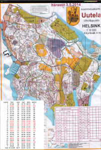
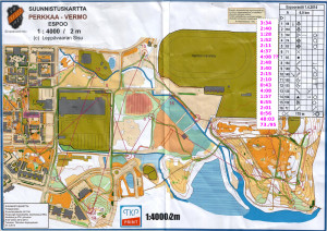
#2, bad (easy!) right-ish direction out of #1
#10 too high up the hill from #9 (which was also hard to find)
#11 slow walking up the hill
#12 down to the path and round the steep cliff - maybe straighter would have been better?
#14 OK "on the map" around the forbidden area, but then drifted left down the hill. worst split 🙁
#15 ok orienteering just too slow..
#19 well hidden control on steep downslope
#21 drifting left into the woods when there would have been a straight path
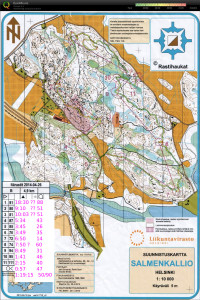
Itärastit Salmenkallio
#1 lots of problems with mistaking one path for the other as well as not knowing which big stone on the map is which in reality
#2 looping close to the control circle - should have a good secure plan all the way to the control
#3 no real route plan and as a result a completely crazy path up&down a big hill. the paths to the left would have been much better probably.
#4, #5, #6, and #7 went OK with #7 being the best split, mostly running on compass-bearing on top of the hill - checking progress form stones/shapes on the map.
#8 drifted too much to the right and going down the steep hill was slow. a bit of hesitation close to the control.
#9, #10, #11 OKish.
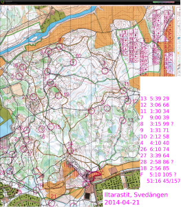
Iltarastit, Svedängen
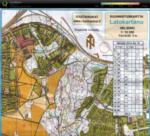
Itärastit, Latokartano
Espoorastit, Vermo
Simple Trajectory Generation
The world is full of PID-loops, thermostats, and PLLs. These are all feedback loops where we control a certain output variable through an input variable, with a more or less known physical process (sometimes called "plant") between input and output. The input or "set-point" is the desired output where we'd like the feedback system to keep our output variable.
Let's say we want to change the set-point. Now what's a reasonable way to do that? If our controller can act infinitely fast we could just jump to the new set-point and hope for the best. In real life the controller, plant, and feedback sensor all have limited bandwidth, and it's unreasonable to ask any feedback system to respond to a sudden change in set-point. We need a Trajectory - a smooth (more or less) time-series of set-point values that will take us from the current set-point to the new desired value.
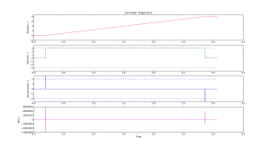
Here are two simple trajectory planners. The first is called 1st order continuous, since the plot of position is continuous. But note that the velocity plot has sudden jumps, and the acceleration & jerk plots have sharp spikes. In a feedback system where acceleration or jerk corresponds to a physical variable with finite bandwidth this will not work well.
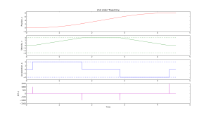
We get a smoother trajectory if we also limit the maximum allowable acceleration. This is a 2nd order trajectory since both position and velocity are continuous. The acceleration still has jumps, and the jerk plot shows (smaller) spikes as before.
Here is the python code that generates these plots:
1 2 3 4 5 6 7 8 9 10 11 12 13 14 15 16 17 18 19 20 21 22 23 24 25 26 27 28 29 30 31 32 33 34 35 36 37 38 39 40 41 42 43 44 45 46 47 48 49 50 51 52 53 54 55 56 57 58 59 60 61 62 63 64 65 66 67 68 69 70 71 72 73 74 75 76 77 78 79 80 81 82 83 84 85 86 87 88 89 90 91 92 93 94 95 96 97 98 99 100 101 102 103 104 105 106 107 108 109 110 111 112 113 114 115 116 117 118 119 120 121 122 123 124 125 126 127 128 129 130 131 132 133 134 135 136 137 138 139 140 141 142 143 144 145 146 147 148 149 150 151 152 153 154 155 156 157 158 159 160 161 162 163 164 165 166 167 168 169 170 171 172 173 174 175 176 177 178 179 180 181 182 183 184 185 186 187 188 189 190 191 192 193 194 195 196 | # AW 2014-03-17 # GPLv2+ license import math import matplotlib.pyplot as plt import numpy # first order trajectory. bounded velocity. class Trajectory1: def __init__(self, ts = 1.0, vmax = 1.2345): self.ts = ts # sampling time self.vmax = vmax # max velocity self.x = float(0) # position self.target = 0 self.v = 0 # velocity self.t = 0 # time self.v_suggest = 0 def setTarget(self, T): self.target = T def setX(self, x): self.x = x def run(self): self.t = self.t + self.ts # advance time sig = numpy.sign( self.target - self.x ) # direction of move if sig > 0: if self.x + self.ts*self.vmax > self.target: # done with move self.x = self.target self.v = 0 return False else: # move with max speed towards target self.v = self.vmax self.x = self.x + self.ts*self.v return True else: # negative direction move if self.x - self.ts*self.vmax < self.target: # done with move self.x = self.target self.v = 0 return False else: # move with max speed towards target self.v = -self.vmax self.x = self.x + self.ts*self.v return True def zeropad(self): self.t = self.t + self.ts def prnt(self): print "%.3f\t%.3f\t%.3f\t%.3f" % (self.t, self.x, self.v ) def __str__(self): return "1st order Trajectory." # second order trajectory. bounded velocity and acceleration. class Trajectory2: def __init__(self, ts = 1.0, vmax = 1.2345 ,amax = 3.4566): self.ts = ts self.vmax = vmax self.amax = amax self.x = float(0) self.target = 0 self.v = 0 self.a = 0 self.t = 0 self.vn = 0 # next velocity def setTarget(self, T): self.target = T def setX(self, x): self.x = x def run(self): self.t = self.t + self.ts sig = numpy.sign( self.target - self.x ) # direction of move tm = 0.5*self.ts + math.sqrt( pow(self.ts,2)/4 - (self.ts*sig*self.v-2*sig*(self.target-self.x)) / self.amax ) if tm >= self.ts: self.vn = sig*self.amax*(tm - self.ts) # constrain velocity if abs(self.vn) > self.vmax: self.vn = sig*self.vmax else: # done (almost!) with move self.a = float(0.0-sig*self.v)/float(self.ts) if not (abs(self.a) <= self.amax): # cannot decelerate directly to zero. this branch required due to rounding-error (?) self.a = numpy.sign(self.a)*self.amax self.vn = self.v + self.a*self.ts self.x = self.x + (self.vn+self.v)*0.5*self.ts self.v = self.vn assert( abs(self.a) <= self.amax ) assert( abs(self.v) <= self.vmax ) return True else: # end of move assert( abs(self.a) <= self.amax ) self.v = self.vn self.x = self.target return False # constrain acceleration self.a = (self.vn-self.v)/self.ts if abs(self.a) > self.amax: self.a = numpy.sign(self.a)*self.amax self.vn = self.v + self.a*self.ts # update position #if sig > 0: self.x = self.x + (self.vn+self.v)*0.5*self.ts self.v = self.vn assert( abs(self.v) <= self.vmax ) #else: # self.x = self.x + (-vn+self.v)*0.5*self.ts # self.v = -vn return True def zeropad(self): self.t = self.t + self.ts def prnt(self): print "%.3f\t%.3f\t%.3f\t%.3f" % (self.t, self.x, self.v, self.a ) def __str__(self): return "2nd order Trajectory." vmax = 3 # max velocity amax = 2 # max acceleration ts = 0.001 # sampling time # uncomment one of these: #traj = Trajectory1( ts, vmax ) traj = Trajectory2( ts, vmax, amax ) traj.setX(0) # current position traj.setTarget(8) # target position # resulting (time, position) trajectory stored here: t=[] x=[] # add zero motion at start and end, just for nicer plots Nzeropad = 200 for n in range(Nzeropad): traj.zeropad() t.append( traj.t ) x.append( traj.x ) # generate the trajectory while traj.run(): t.append( traj.t ) x.append( traj.x ) t.append( traj.t ) x.append( traj.x ) for n in range(Nzeropad): traj.zeropad() t.append( traj.t ) x.append( traj.x ) # plot position, velocity, acceleration, jerk plt.figure() plt.subplot(4,1,1) plt.title( traj ) plt.plot( t , x , 'r') plt.ylabel('Position, x') plt.ylim((-2,1.1*traj.target)) plt.subplot(4,1,2) plt.plot( t[:-1] , [d/ts for d in numpy.diff(x)] , 'g') plt.plot( t , len(t)*[vmax] , 'g--') plt.plot( t , len(t)*[-vmax] , 'g--') plt.ylabel('Velocity, v') plt.ylim((-1.3*vmax,1.3*vmax)) plt.subplot(4,1,3) plt.plot( t[:-2] , [d/pow(ts,2) for d in numpy.diff( numpy.diff(x) ) ] , 'b') plt.plot( t , len(t)*[amax] , 'b--') plt.plot( t , len(t)*[-amax] , 'b--') plt.ylabel('Acceleration, a') plt.ylim((-1.3*amax,1.3*amax)) plt.subplot(4,1,4) plt.plot( t[:-3] , [d/pow(ts,3) for d in numpy.diff( numpy.diff( numpy.diff(x) )) ] , 'm') plt.ylabel('Jerk, j') plt.xlabel('Time') plt.show() |
See also:
- EMC2 tpRunCycle revisited and the correspoinding LinuxCNC wiki page
- Lambrechts 2004 paper, with step by step instructions for generating a 4th order trajectory.
- or a longer report by Lambrecht on the same subject
I'd like to extend this example, so if anyone has simple math+code for a third-order or fourth-order trajectory planner available, please publish it and comment below!
ADF4350 PLL+VCO and AD9912 DDS power spectra
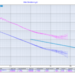
Update 2015-09-28: ADEV and Phase-noise measured with a 3120A:
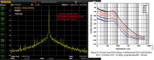
Here's the 1 GHz output of an ADF4350 PLL+VCO evaluation board, when used with a 25 MHz reference.
The datasheet shows a phase noise of around -100 dBc/Hz @ 1-100 kHz, so this measurement may in fact be dominated by the Rigol DSA1030A phase noise which is quoted as -88 dBc/Hz @ 10 kHz.
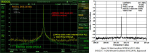
The 1 GHz output from the ADF4350 is used as a SYCLK input for an AD9912 DDS. The spectrum below shows a 100 MHz output signal from the DDS with either a 660 MHz or 1 GHz SYSCLK. The 660 MHz SYSCLK is from a 10 MHz reference multiplied 66x by the AD9912 on-board PLL. The 1 GHz SYSCLK is from the ADF4350, with the AD9912 PLL disabled.
The AD9912 output is clearly improved when using an external 1 GHz SYSCLK. The noise-floor drops from -80 dBm to below -90 dBm @ 250 kHz from the carrier. The spurious peaks at +/- 50 kHz disappear. However this result is still far from the datasheet result where all noise is below -95 dBm just a few kHz from the carrier. It shouldn't matter much that the datasheet shows a 200MHz output while I measured a 100 MHz output.
Again I suspect the Rigol DSA1030A's phase-noise performance of -88dBc/Hz @ 10 kHz may in fact significantly determine the shape of the peak. Maybe the real DDS output is a clean delta-peak, we just see it like this with the spectrum analyzer?
Martein/PA3AKE has similar but much nicer results over here: 1 GHz refclock and 14 MHz output from AD9910 DDS. Amazingly both these spectra show a noise-floor below -90 dBm @ 50 Hz! Maybe it's because the spectrum analyzer used (Wandel & Goltermann SNA-62) is much better?
DDS Front Panel
Two of these 1U 19" rack-enclosure front panels came in from Shaeffer today. Around 70 euros each, and the best thing is you get an instant quote on the front panel while you are designing it with their Front Panel Designer software. The box will house an AD9912 DDS.
From left to right: 10 MHz reference frequency input BNC, DDS output BNC, 40mm fan (1824257 and 1545841), 20x2 character LCD (73-1289-ND), rotary encoder with pushbutton (102-1767-ND), and rightmost an Arduino Due (1050-1049-ND) with Ethernet shield (1050-1039-ND). The panel is made to fit a Schroff 1U enclosure (1816030) with the inside PCBs mounted to a chassis plate (1370461).
Here's a view from the inside. I milled down the panel thickness from 4 mm to around 2.5 mm on the inside around the rotary encoder. Otherwise all components seem to fit as designed.
Next stop is coding an improved user-interface as well as remote-control of the DDS and PLL over Ethernet.
Drop-Cutter toroid edge test
The basic CAM-algorithm called axial tool projection, or drop-cutter, works by dropping down a cutter along the z-axis, at a chosen (x,y) location, until we make contact with the CAD model. Since the CAD model consists of triangles, drop-cutter reduces to testing cutters against the triangle vertices, edges, and facets. The most advanced of the basic cutter shapes is the BullCutter, a.k.a. Toroidal cutter, a.k.a. Filleted endmill. On the other hand the most involved of the triangle-tests is the edge test. We thus conclude that the most complex code by far in drop-cutter is the torus edge test.
The opencamlib code that implements this is spread among a few files:
- millingcutter.cpp translates/rotates the geometry into a "canonical" configuration with CL=(0,0), and the P1-P2 edge along the X-axis.
- bullcutter.cpp creates the correct ellipse, calls the ellipse-solver, returns the result
- ellipse.cpp ellipse geometry
- ellipseposition.cpp represents a point along the perimeter of the ellipse
- brent_zero.hpp has a general purpose root-finding algorithm
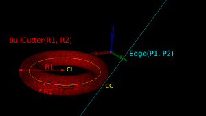
The special cases where we contact the flat bottom of the cutter, or the cylindrical shaft, are easy to deal with. So in the general case where we make contact with the toroid the geometry looks like this:
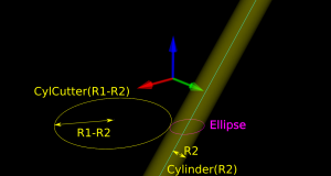
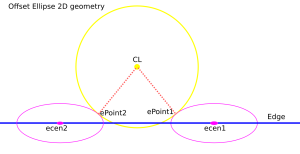
Here we've fixed the XY coordinates of the cutter location (CL) point, and we're using a filleted endmill of radius R1 with a corner radius of R2. In other words R1-R2 is the major radius and R2 is the minor radius of the Torus. The edge we are testing against is defined by two points P1 and P2 (not shown). The location of these points doesn't really matter, as we do the test against an infinite line through the points (at the end we check if CC is inside the P1-P2 edge). The z-coordinate of CL is the unknown we are after, and we also want the cutter contact point (CC).
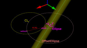
There are many ways to solve this problem, but one is based on the offset ellipse. We first realize that dropping down an R2-minor-radius Torus against a zero-radius thin line is actually equivalent to dropping down a zero-minor-radius Torus (a circle or 'ring' or CylCutter) against a R2-radius edge (the edge expanded to an R2-radius cylinder). If we now move into the 2D XY plane of this circle and slice the R2-radius cylinder we get an ellipse:
The circle and ellipse share a common virtual cutter contact point (VCC). At this point the tangents of both curves match, and since the point lies on the R1-R2 circle its distance to CL is exactly R1-R2. In order to find VCC we choose a point along the perimeter of the ellipse (an ellipse-point or ePoint), find out the normal direction, and go a distance R1-R2 along the normal. We arrive at an offset-ellipse point (oePoint), and if we slide the ePoint around the ellipse, the oePoint traces out an offset ellipse.
Now for the shocking news: an offset-ellipse doesn't have any mathematically convenient representation that helps us solve this!
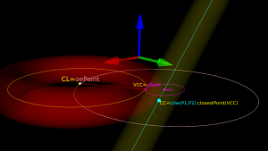
Instead we must numerically find the best ePoint such that the oePoint coincides with CL. Like so:
Once we've found the correct ePoint, this locates the ellipse along the edge and the Z-axis - and thus CL and the cutter . If we go back to looking at the Torus it is obvious that the real CC point is now the point on the P1-P2 line that is closest to VCC.
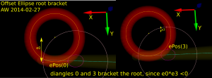
In order to run Brent's root finding algorithm we must first bracket the root. The error we are minimizing is the difference in Y-coordinate between the oePoint and the CL point. It turns out that oePoints calculated for diangles of 0 and 3 bracket the root. Diangle 0 corresponds to the offset normal aligned with the X-axis, and diangle 3 to the offset normal aligned with the Y-axis:
Finally a clarifying drawing in 2D. The ellipse center is constrained to lie on the edge, which is aligned with the X-axis, and thus we know the Y-coordinate of the ellipse center. What we get out of the 2D computation is actually the X-coordinate of the ellipse center. In fact we get two solutions, because there are two ePoints that match our requirement that the oePoint should coincide with CL:
Once the ellipse center is known in the XY plane, we can project onto the Edge and find the Z-coordinate. In drop-cutter we obviously approach everything from above, so between the two potential solutions we choose the one with a higher z-coordinate.
The two ePoint solutions have a geometric meaning. One corresponds to a contact between the Torus and the Edge on the underside of the Torus, while the other solution corresponds to a contact point on the topside of the Torus:
I wonder how this is done in the recently released pycam++?
OpenCAMlib and OpenVoronoi toolpath examples
There might be renewed hope for a FreeCAD CAM module. Here are some examples of what opencamlib and openvoronoi can do currently.
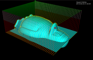
The drop-cutter algorithm is the oldest and most stable. This shows a parallel finish toolpath but many variations are possible.
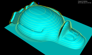
The waterline algorithm has some bugs that show up now and then, but mostly it works. This is useful for finish milling of steep areas for the model. A smart algorithm would use paralllel finish on flat areas and waterline finish on steep areas. Another use for the waterline algorithm is "terrace roughing" where the waterline defines a pocket at a certain z-height of the model, and we run a pocketing path to rough mill the stock at this z-height. Not implemented yet but doable.
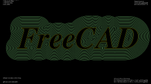
This shows offsets calculated with openvoronoi. The VD algorithm is fairly stable for input geometries with line-segments, but some corner cases still cause problems. It would be nice to have arc-segments as input also, but this requires additional work.
The VD is easily filtered down to a medial-axis, more well-known as a V-carving toolpath. I've demonstrated this for a 90-degree V-cutter, but toolpath is easy to adapt for other angles. Input geometry comes from truetype-tracer (which in turn uses FreeType).
Finally there is an experimental advanced pocketing algorithm which I call medial-axis-pocketing. This is just a demonstration for now, but could be developed into an "adaptive" pocketing algorithm. These are the norm now in modern CAM packages and the idea is not to overload the cutter in corners or elsewhere - take multiple light passes instead.
The real fun starts when we start composing new toolpath strategies consisting of many of these simple/basic ones. One can imagine first terrace-roughing a part using the medial-axis-pocketing strategy, then a semi-finish path using a smart shallow/steep waterline/parallel-finish algorithm, and finally a finish operation or even pencil-milling.
