En motorbåt körde på Skåldö färjans vajer ca 19:30 tiden. Alla ombord verkade ha klarat sig utan större skador och fördes bort med ambulans. Motorbåten satt fast i vajern och brandkår + färj-kapten försökte först få loss båten, men det slutade med att färjan togs loss från vajern och båt+vajer sjönk till bottnen! Färj trafiken löpte normalt igen ca 20:45.
Här en animation där man ser båten sjunka: farjan_animation2 (5 Mb AVI-fil)
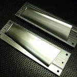
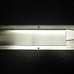
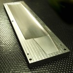
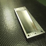
With the servo-upgrade of the cnc-mill complete we are now beginning to run the kind of jobs that weren't previously possible. Stepper motors simply don't give the kind of 3D contouring capability and reliability for running 3-4 hour finish jobs like these. The finmould is finished with a 6 mm ball-nose cutter.
Jari made these moulds in steel, but it's possible to cut them in aluminium too. The fin mould here has a NACA 0010 section and the rudder has a thicker NACA 0015 section. With the precision that cnc-cutting provides we hope that the fin can come out of the mould quite complete and fit a cnc-cut finbox/bulb without much manual fitting.
We can produce fin, rudder, and bulb moulds in steel or aluminium on a small scale. Get in touch by email or by commenting below if you are an interested IOM-builder.
In an attempt to image the acoustic fields emerging from ultrasound transducers we've built a small Schlieren setup with stroboscopic LED illumination. There's a 10-cycle 7.5 MHz sound-wave coming in from the top at a velocity of around 1500 m/s, and if you illuminate it at just the right time with a 500 ns pulse of light you see the change in refractive index due to the pressure change. In the videos we are adjusting the delay between the acoustic pulse and the light-pulse from about 0 us up to 10 us to see how the sound propagates through the ~15 mm field of view.
Here's another one with a reflecting metal piece at the bottom. The reflected pulse shows quite nicely! If you look carefully between 3 and 4 s you can see an interference pattern between the incoming and reflected pulse.
As I'm very much an amateur programmer with not too much time to learn new stuff I've decided my CAM-algorithms are going to be written in Python (don't hold your breath, they'll be online when they'll be online...). The benefits of rapid development will more than outweigh the performance issues of Python at this stage.
But then I found Mark Dufour's project shedskin (see also blog here and Mark's MSc thesis here), a Python to C++ compiler! Can you have the best of both worlds? Develop and debug your code interactively with Python and then, when you're happy with it, translate it automagically over to C++ and have it run as fast as native code?
Well, shedskin doesn't support any and all python constructs (yet?), and only a limited number of modules from the standard library are supported. But still I think it's a pretty cool tool. For someone who doesn't look forward to learning C++ from the ground up typing 'shedskin -e myprog.py' followed by 'make' is just a very simple way to create fast python extensions! As a test, I ran shedskin on the pystone benchmark and called both the python and c++ version from my multiprocessing test-code:
The people at EMC2 Fest (webcam here) made this AVI of 5-axis machining a sphere using some custom g-code and povray.
I've been playing around with vpython, so you can expect some CAM-related posts on drop-cutter in Python and associated 3D views or animations in the not too distant future.
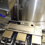
Here's a setup wit three vises for machining model yacht tiller arms. The parts are rotated 90 degrees between the first stage (leftmost) and the second stage (middle), and then again 90 degrees for the final stage (right). There's some rigid tapping at around 8:20.
Optical tweezers use light to trap dielectric particles in an approximately harmonic potential. If the position of the bead is X, the position of the trap Xtrap, and the stiffness of the trap k then the equation of motion looks like this:
where Beta is the drag coefficient and Ft is a random white-noise thermal force (the bead is so small that kicks and bumps by surrounding water-molecules matter!). If the trap stays in one place all the time (Xtrap is constant) the power-spectral-density (PSD) of the bead fluctuations turns out to be Lorentzian.
But if there's a fast way of steering the trap, we might try feedback control where we actively steer Xtrap based on some feedback signal:
This is a position-clamp where we use proportional feedback with gain Kp to keep the bead bead at some fixed set-point Xset. Tau accounts for some delay in measuring the bead position and in steering the trap. Inspired by a magnetic-tweezers paper by Gosse et al. we inserted this into the equation of motion to find the PSD:
So how do we go about verifying this experimentally? Well, you build something like this:
The idea is to use a powerful laser at 1064 nm for trapping. It can be steered with about a 10 us delay using AODs. Then we use another laser at 830 nm to detect the position of the trapped particle using back-focal-plane interferometry. But since in-loop measurements in feedback loops can give funny results it's best to verify the position measurement with a third laser at 785 nm. The feedback control is performed by a PCI-7833R DAQ card from National Instruments which houses an AD converter for reading in the position signals at 200 kS/s and 16-bit precision, and then we do the feedback algorithm on a 3 Mgate FPGA. We output the steering command as 30 bit numbers in parallel to DDSs that drive the AODs. The 10 us delay in the AOD (the acoustic time-of-flight in the crystal) combined with the AD-conversion time of 5 us gives a total loop-delay of around 15 us in our setup.
It all works quite nicely! The colored PSD traces are experimental data at increasing feedback gain starting from the blue trace at the top (zero gain, Lorentzian shape as expected) down to the black trace at the bottom (gain 24.8). When increasing the gain further trapping becomes unstable due to the peak at ~12 kHz (think about what's usually termed 'feedback': pointing a microphone at a loudspeaker). The theoretical PSDs are shown as solid lines and they agree pretty well with the experiment. The inset shows the effective trap stiffness calculated from the integral of the PSD. We're able to increase the lateral effective trap stiffness around 10-13 fold compared to the no-feedback situation.
This video shows a time-series of the bead position (left) and the trap position (right) first with no feedback where we see the bead fluctuating a lot and the trap stationary, and then with feedback gain applied (gain=7) where we see the bead-noise significantly reduced and the trap moving around.
These results appear as a 3-page write-up in today's Applied Physics Letters:
We're not the first ones to perform this experiment, but I would argue that our paper is the first one to do all steps in the experiment properly, and we get the nice agreement between theory and experiment.
An early paper by Simmons et al. claims a 400-fold improvement in effective trap stiffness using an analog feedback circuit. There's no discussion about the feedback bandwidth or the PSD when position-clamping. Perhaps a case of undersampling?
Simulations by Ranaweera et al. indicate that a 65-fold increase in effective trap stiffness can be achieved, but there's no discussion about how the delays in the feedback loop affect this, and there's no experimental verification.
More recently, Wulff et al. used steering mirrors to do the same thing, but they used the position detection signal from the trapping laser itself for feedback control. I'm not sure what this achieves since the coordinate-system in which you do position measurements is going to be steered around as you try to minimize fluctuations. Their PSDs don't look like ours, and the steering mirror has a bandwidth of only a few hundred Hz so you cannot control the high frequency noise like this.
Increasing the stiffness of optical tweezers by other means seems like a fashionable topic. A recent paper from Alfons van Blaaderen's group uses counter propagating beams to trap high-index (n>2) particles effectively, while simulations by Halina Rubinsztein-Dunlop's group indicate that anti-reflection coating the beads also improves trapping efficiency.
By popular demand, some details on the spindle, spindle-motor, and VFD of our cnc-mill which just recently was able to do rigid-tapping.
The motor is a standard induction motor from ABB rated at 1.5 kW and around 3000 rpm (at 50 Hz AC). It has a lot of model identification numbers: "1.5 kW M2VA 80 C-2 3G Va 08 1003-CSB ". There are more details on this line of motors on ABB's site, but this kind of motor should be available from almost any manufacturer of industrial induction motors. Presumably torque drops off after the rated maximum rpm of 3000, but with small diameter tools we have been running the VFD up to 90 Hz or around 5400 rpm. When taking heavy cuts the VFD tries its best to keep the rpm up, but we do observe a 100-200 rpm drop when a 40 mm face-mill digs in. It might be possible to wire the encoder counts to the VFD and get a truly closed loop system but I doubt it's worth it.
The motor is connected to an Omron Varispeed V7 VFD with a maximum motor capacity of 1.5 kW. I can't find a good link on the international Omron site, so here's one in finnish instead (datasheet here). This is a sensorless vector-drive VFD, which is very important - with the previous simple V/f open-loop VFD we could only do machining close to maximum RPM and certainly would not have tried rigid-tapping. The electrical connection is simple with the VFD connecting to 1-phase AC mains and then the three phases from the VFD connecting to the motor.
The VFD is controlled by EMC2 using three general purpose IO pins on the m5i20. One pin sets the rpm (VFD reference frequency) using a pulse-train generated by the stepgen HAL component (step_type=2 ctrl_type=v). The two other IO lines set the VFD to either forward or reverse.
Below a close-up of the US Digital 500 ppr encoder mounted on top of the motor. There's a cooling fan driven by the main motor axle on top of the motor and we tapped the axle with a M6 thread, inserted an M6 set-screw, and coupled the set-screw to the encoder using plastic tubing. The encoder sits on a alu-bracket which is bolted to the fan grille. Z-axis servo in the background.