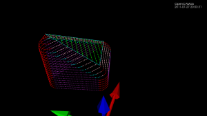
Threading and OpenGL, test 2

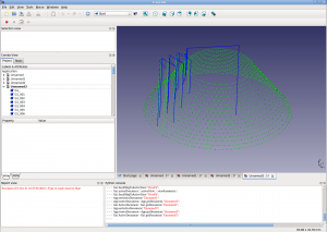
Here's a simple test program using LibQGLViewer (screen capture with xvidcap). The vertex array and the index array that OpenGL draws (using glDrawElements) are held in a GLData class which holds a mutex. The Viewer class locks the mutex while drawing, and the worker-thread locks the mutex while updating the data. Here the worker task re-positions the original vertex position, signals the Viewer to draw, and then sleeps for 40 ms. When we don't rotate or zoom with the mouse the frame-rate should thus be 25 Hz. Rotating or zooming causes more frequent re-draws and a higher frame-rate.

To gain any real benefit on a multi-core machine I think the worker thread needs to work on a 'dirty' copy of the data, and we only lock the mutex for a minimal time while swapping in the updated data for the real data. Anyone have any good example code for this? Both a case where the worker produces new data at a slow rate (slower than Viewer re-draws), and at a faster rate should be handled.

Here's an UML(ish) diagram drawn with dia:

Code.

Multithreaded OpenGL with Qt

I've looked at this example from 2003 and converted it to something that compiles with qt4.7. Here: https://github.com/aewallin/sandbox/tree/master/qt_opengl_threads

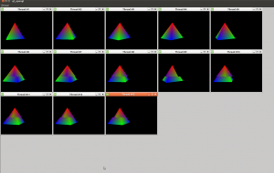
Each window is a QGLWidget with its own QThread associated with it that does the drawing. That means the UI should stay responsive despite heavy processing in the threads.

I wonder if this can be made to work with libQGLViewer ?


(The screenshot has caught many windows in the middle of a drawing operation. I couldn't get double-buffering to work. In practice it looks very smooth to the eye.)

Cutsim driven by g-code

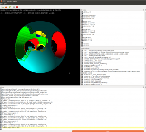
Based on Mark Pictor's cam-occ work I've been able to use the emc2 g-code interpreter 'rs274' binary that gets built during an emc2-build. It reads g-code files and outputs 'canonical' motion commands (see e.g. "The NIST RS274/NGC Interpreter - Version 3"). I'm positioning the tool at densely sampled points along each move, and subtracting it from the stock (see Yau and Yau) . The stock model is a distance field stored in an adaptive octree (see Frisken and Frisken).

This is very experimental: There's one kind of stock and one kind of tool, namely spherical!, The stock and tool sizes and colors are hard-coded, There's only one thread which means the UI becomes unresponsive and greyed-out during about 57s of processing. It's slow, 57s for a fairly simple 20-line g-code file. We assume hard-coded paths for the 'rs274' binary and the emc2 tooltable-file.

Octree operations

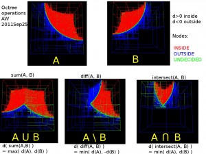
I've looked at set-operations (union, difference, intersection) for octrees again. Previously I tried it with linear-octrees and visualization with python and VTK. Now I'm using a traditional pointer-based octree data-structure, and drawing with OpenGL VBOs. With the addition of a g-code interpreter, a user-interface, and an isosurface extraction algorithm (such as marching-cubes) this should converge towards a milling/turning/3d-printing cutting-simulation sometime soon...

References: Frisken2000 and Frisken2006.

vd benchmark

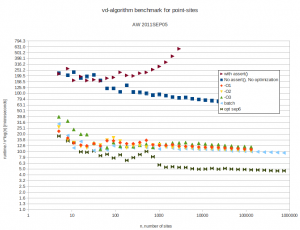
Tuesday update: A few optimizations has shaved about half off the constant, to . This was mainly (a) choosing boost::vecS as the out-edge container for the BGL-graph, and (b) choosing std::vector instead of std::set for a temporary variable in the grid-search for the closest facet. I suspect the runtime is dominated by that grid-search. Profiling would tell.

I did some benchmarking of my vd-code. It is supposed to run in time. Benchmarking turns out to be not so simple. I normally compile without any optimizations, and with a lot of sanity-checks and assert():s all over the code. These checks have worse time-complexity and result in long runtimes with big inputs. Then there are compiler optimization flags like -O or -O3.

I was first running the algorithm by inserting each point from python-code:

    t_before = time.time()
    for p in plist:
        vd.addVertexSite( p )
    t_after = time.time()
    return (t_after - t_before)

which I thought could add some overhead. I also made a version ("batch mode") where we first push all points to c++, and then call a run() method:

    for p in plist:
        vd.pushVertexSite( p )
    t_before = time.time()
    vd.run()
    t_after = time.time()
    return (t_after - t_before)

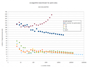
but this seems to improve runtime only marginally. Here are the results. Runtimes are divided by , so ideally all points should fall on a horizontal line. At best the code now runs in about 10-16 microseconds times .

With 4096 input points the runtime improves from 12s down to 1.3s by turning off sanity-checks and assert():s. It further improves to 0.18s with -O3 and to 0.165s in batch-mode.

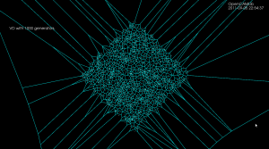
As an example, the voronoi diagram for 1000 random points looks like this:

Line-segment voronoi diagram notes

The next step for the opencamlib voronoi-diagram (vd) algorithm is to be able to add line-segment generators. Some notes and ideas on that then (this turned into a rather long post...)

First let's recall (from February) how the point-generator vd-algorithm works:
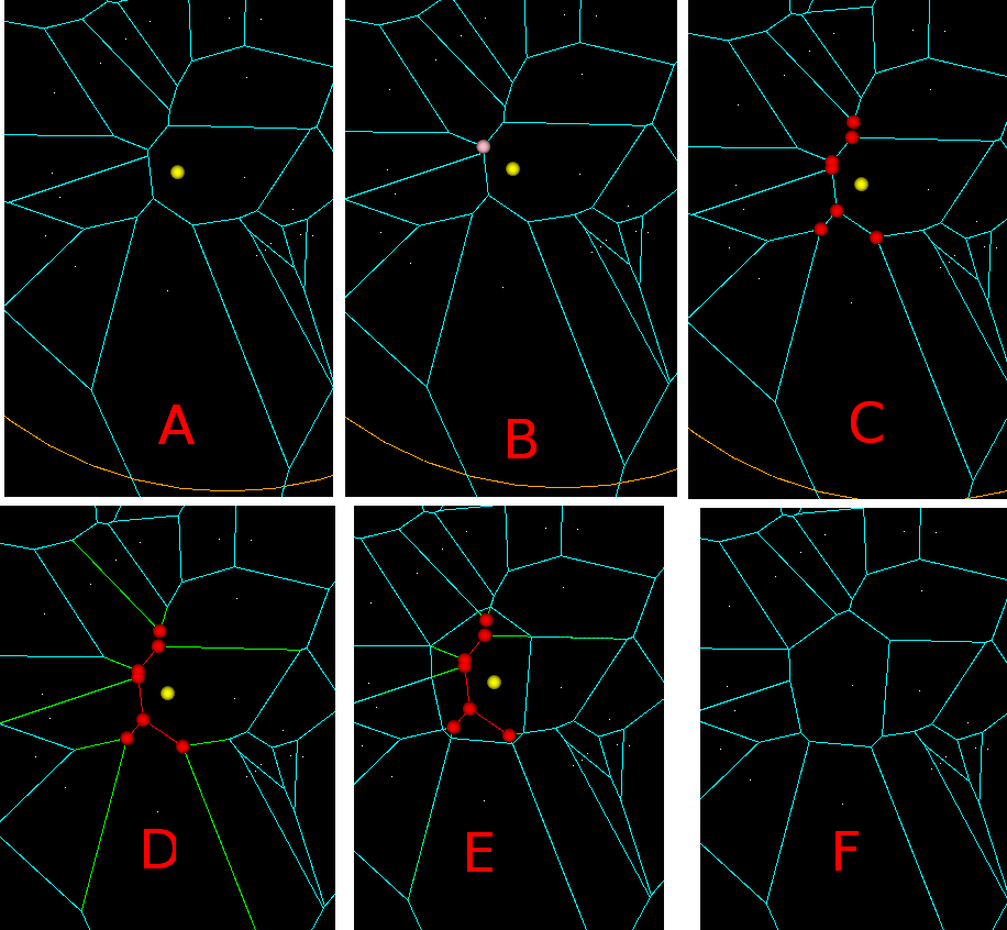
In (A) we want to insert a new point-generator (yellow). First we need to identify the closest point-generator among the existing generators. (B) Then among the vertices that bound this voronoi-face(region) we search for a seed vertex (pink). The seed vertex is the one that violates the inCircle-predicate the most, i.e. has the minimum distance to the new point-to-be-inserted. (C) Starting from the seed vertex, we then identify other vertices (red) that need to be deleted, because they are closer to the new generator than to any other generator. These vertices are called "IN" vertices, and the associated edges (also in red) should (i) form a tree (a connected acyclic graph) and (ii) for any face, the "IN"-vertices should be connected, and the "OUT" vertices should be connected. (D) IN-IN edges (red) will be deleted completely, while NEW vertices will be generated on each IN-OUT edge (green). (E) NEW-NEW edges are created and connected into a cycle which forms the face/region for the new generator. (F) Now all IN-vertices and all IN-IN as well as IN-NEW edges are deleted and we are done.

Now the case when we insert a line segment. We start as above by constructing the diagram for all point-generators as well as all the endpoints of our line-segments. Here is an image from the Sugihara&Iri 2000 paper (http://dx.doi.org/10.1007/s004530010002) which I have enhanced with colors and text.
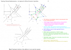
The steps of the algorithm are similar to (A)-(F) above: In (A), since we have already inserted the two endpoints of the line-segment, we obviously know in which face to look for the seed-vertex. (B) when we search for a seed-vertex we now need both a dist(VDVertex, PointGenerator) function and a dist(VDVertex, LineGenerator) function. In (C) we again expand the set of "IN" vertices (red circles), while keeping the associated graph a tree, and not disconecting "IN"-vertices or "OUT"-vertices of any face (i and ii above) .

A new (iii) requirement is that the tree should connect the regions of the line-segment endpoints. A new situation also appears where the two endpoints of an edge are classified as "IN", but the complete edge should not be deleted. This is because edges between point and line-segment generators are parabolic arcs (curved!). In this case two NEW vertices are generated on the edge, so it splits into three parts: IN-NEW, NEW-NEW, and NEW-IN. This needs to be dealt with, but I'm not sure exactly how. I think one of the Held papers talks about avoiding this special case by splitting each parabolic edge in two, at the "vertex" of the parabola i.e. the point of greatest curvature (?).

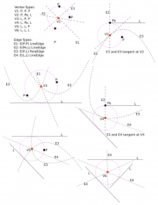
"IN-IN" edges (magenta) will again be deleted. (D) NEW-vertices (green) should now be generated on each IN-OUT edge. This needs new functionality, since we need to deal with two types of edges: LineEdge and ParabolicEdge. The LineEdge occurs between two PointGenerators or between two LineGenerators, while the ParabolicEdge appears between a PointGenerator and a LineGenerator. The NEW vertex we need to generate will obviously be located on the IN-OUT edge (with associated generators gen1, gen2), and should be positioned so that it is equidistant from gen1, gen2, and the new line-segment generator. In contrast to the old point-generator diagram code where we only had one type of VDVertex, namely VDVertex( PointGenerator, PointGenerator, PointGenerator), we now have 6 (six!) different types of vertices in the diagram, depending on the three neighbouring generators, which can be of type LineGenerator, PointGenerator(endpoint), or PointGenerator:

  • VDVertex( PointGenerator, PointGenerator, PointGenerator), type V1 in Okabe et al.
  • VDVertex( PointGenerator, PointGenerator(endpoint) , LineGenerator), type V2
  • VDVertex( LineGenerator, PointGenerator, PointGenerator), type V3
  • VDVertex( LineGenerator, LineGenerator, PointGenerator(endpoint) ),  type V4
  • VDVertex( LineGenerator, LineGenerator, PointGenerator ), type V5
  • VDVertex( LineGenerator, LineGenerator, LineGenerator ), type V6

When these NEW-vertices (green) have been created, the next step is to connect them into a cycle with NEW-NEW edges (green). As we loop around the face we need to create either LineEdges or ParabolicEdges, depending on the neighbouring generators. Okabe lists the four different types of edges that appear in the diagram:

  • VDEdge( PointGenerator, PointGenerator), type E1 (LineEdge)
  • VDEdge( PointGenerator(endpoint), LineGenerator), type E2 (LineEdge)
  • VDEdge( PointGenerator, LineGenerator), type E3 (ParabolicEdge)
  • VDEdge( LineGenerator, LineGenerator), type E4 (LineEdge)

That's about it. It shouldn't be that hard to modify the current code to allow for six types of different VDVertex and four different types of VDEdge, and come up with a suitable design-pattern so that the correct type of vertex and edge are generated based on the type of the generators. Stay tuned...

Update1: here is another image with the same color-coding, from the Held VRONI-paper. The orange edge illustrates a case where the edge is marked "IN-IN" but in fact two new vertices should be generated on it, and the NEW-NEW portion of the edge is retained in the updated diagram (on the right).
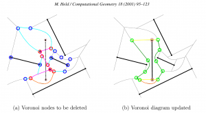
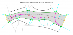
Update2: Here is an image from the Held 2009 paper, which describes VDs for line-segment and circular arc generators. The circular arcs add a few additional special cases and some complexity, but the core of the algorithm remains the same: (1) find a seed vertex, (2) expand the set of 'marked' or "IN" vertices maximally, while keeping IN-IN edges (red) a tree, (3) generate NEW vertices (green) on IN-OUT edges (cyan), (4) hook up the NEW vertices with new edges (green) to form the new voronoi region, (5) delete IN-vertices, IN-IN edges, and IN-NEW edges.
Update3: Here's a drawing which shows the six different types of vertices.
Opencamlib cutter shapes

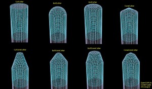
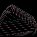
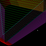
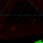
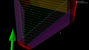
If you calculate toolpaths around a very narrow and 'pointy' triangle you will get toolpaths in the shape of the inverse cutter - the "Inverse Tool Offset". Here I've plotted the basic operations, in red/blue drop-cutter which drops the cutter down along the z-axis until it contacts the triangle, and in cyan waterlines which are the results of a push-cutter operation that pushes the cutter at constant z-height along the x/y axis into contact with the triangle.

There are four basic cutter shapes: (1) Cylinder, (2) Sphere('Ball'), (3) Toroid('Bull'), and (4) Cone. The triangle contact can be divided into tests for contact with (a) the three vertices of the triangle, (b) the facet of the triangle, and (c) the three edges of the triangle. That's 4x3 = 12 contact/collision-test functions that have to be written (a few, particularly the facet-tests, can be combined into one base-class method).

Once the basic cutter shapes work it is possible to combine them through CompositeCutter. The bottom row shows cutters with a central part corresponding to the top row of cutters, and a conical outer part.

The point of this exercise is of course not only to plot inverse-tool-shapes, but to be able to calculate toolpaths for these and other CompositeCutter tool shapes. This will become more interesting if/when the cutting-simulation starts working and it will be possible to compare for example surface-finish vs. cutting-time of a BallCutter operation vs. a BullCutter operation.

Comparing waterlines

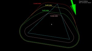
Here's a picture which compares the waterline toolpath for different cutters around a single triangle (cyan). The outermost path (red) is for a cylindrical cutter where we always make contact with either the shaft of the cutter or the circular rim/end of the cutter. Next is the yellow line for the toroidal or BullCutter, followed by the green line for a spherical or BallCutter. The innermost waterline (pink) is for a conical ConeCutter.

waterline_compare

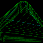
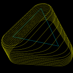
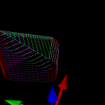
Here are some more waterlines at different heights. This exercise has uncovered at least two new bugs with CylCutter and ConeCutter! The CylCutter seems to fail when asking for a waterline at z=0.0, so that might hint at where the problem is. I'm not sure what is causing the jagged shape with ConeCutter.

Update: The cl-points for conecutter look right, so there must be something strange going on with the weave??

conecutter_looks_ok

Cone-cutter waterlines

I'm not sure why it has taken so long to get the push-cutter methods for ConeCutter written. You would think that the cylindrical, spherical, or toroidal cases are at least as hard. Somehow I have just avoided working on the cone-cutter...

The easy part is as usual contacts between the cutter and the vertices of a triangle - these are shown as red dots. Contact with the facet of the triangle can be made in two ways (1) by the tip of the cone, or (2) by the circular base of the cone, when the facet is steeper than the cone. These are shown in green.

The more involved case is contacts with the edge of the triangle. There are again two cases: We can make contact with the circular base of the cone (cyan dots), or we can make contact with the actual conical part of the cutter (pink dots).
conecutter_00034

Here is an animation that gives the code a workout. Note how the color of the contact-points changes depending both on what part of the triangle we are making contact with and on what part of the cutter is making the contact.

I have now used github for a while, and will probably merge the conecutter feature-branch into master very soon. Almost as soon as I tried github google-code also started supporting git, but possibly the forking and social aspects of github make a switch worthwhile anyway.

There are some interesting developments on the higher level Waterline/Weave algorithm also, which will reduce the memory-consumption of the algorithm from N*N to N+N (where N is the number of Fibers). This will hopefully make Waterline more useful as now many people have been running out of RAM or just seen sudden crashes. Stay tuned...