Temperature PID control - Part Deux

Update: this version of the component may compile on 10.04LTS without errors/warnings: frequency2temperature.comp (thanks to jepler!)

There's been some interest in my 2-wire temperature PID control from 2010. It uses one parallel port pin for a PWM-heater, and another connected to a 555-timer for temperature measurement. I didn't document the circuits very well, but they should be simple to reproduce for someone with an electronics background.

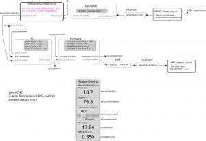
Here's the HAL setup once again:

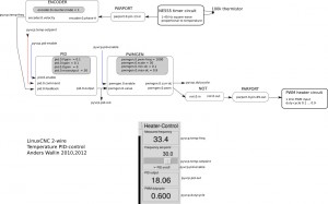
The idea is to count the 555 output-frequency with an encoder, compare this to a set-point value from the user, and use a pid component to drive a pwm-generator that drives the heater.

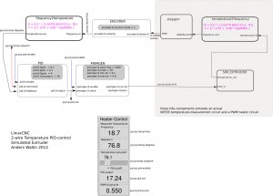
Now it might be nicer to set the temperature in degrees C instead of a frequency. I've hacked together a new component called frequency2temperature that can be inserted after the encoder. This obviously required the thermistor B-parameters as well as the 555-astable circuit component values as input (these are hard-coded constants in frequency2temperature.comp) . Like this:

I didn't have the actual circuits and extruder at hand when coding this. So instead I made a simulated extruder (sim_extruder) component and generated simulated 555-output. Like this:

This also requires a conversion in the reverse direction called temperature2frequency. A stepgen is then used to generate a pulse-train (simulating the 555-output).

  • The INI and HAL files for the simulated extruder, based on the default axis_mm config: simextruder
  • frequency2temperature component:  frequency2temperature.comp (install with: "comp --install frequency2temperature.comp")
  • temperature2frequency component: temperature2frequency.comp (only for simulated setup, not required if you have actual hardware)
  • sim_extruder component: sim_extruder.comp (only for simulated setup, not required if you have actual hardware)

"heartyGFX" has made some progress on this. He has a proper circuit diagram for the PWM-heater and 555-astable. His circuits look much nicer than mine!

The diagrams above were drawn with Inkscape in SVG format: temp_pid_control_svg_diagrams
Why Real-Time?

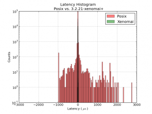
Why bother with these real-time kernels and APIs at all? Isn't timing on a modern PC good enough? Look at this:

This histogram shows latency-numbers from the same 1ms thread test run compiled without (red) and with (green) real-time enabled. All the green real-time data clusters around zero +/- 20us. Without real-time enabled the event we are expecting to happen every 1 ms might happen almost 1 ms too early, or up to 3 ms late. With real-time the timing is mostly consistent to better than 1% (10 us) with a worst-case jitter of 2% (20 us).

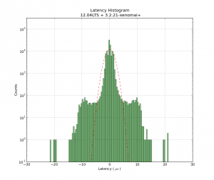
Latency Histogram

This shows a latency-histogram for a 1 ms thread running on Xenomai on my recently acquired ITX-board. Note how badly the histogram is approximated by a normal distribution (Gaussians look like parabolas with logarithmic y-scale!). See also Michael's recent RPi data and  Kent's Athlon/P4 data.

The usual latency-test numbers people report is the maximum latency, a measure of how far out to the left or right the most distant single data point lies. The histrogram can probably be used to extract many more numbers, but for real-time critical applications like cnc-machine control the maximum latency is probably an OK figure of merit.

The latency numbers are recorded with a simple HAL component:lhisto.comp

The instantaneous latency-number is then put in a FIFO by the real-time component sampler and written to a text-file using halsampler. I'm setting this up with the following HAL commands (put this in a file myfile.halrun and run with "halrun -f myfile.halrun")

loadrt threads name1=servo period1=1000000
loadrt sampler depth=1000 cfg=S
loadrt lhisto names=shisto
addf shisto servo
addf sampler.0 servo
net latency shisto.latency sampler.0.pin.0
start
loadusr halsampler -c 0  latencysamples.txt

The numbers can now be plotted with matplotlib. I'm using the following script:

1
2
3
4
5
6
7
8
9
10
11
12
13
14
15
16
17
18
19
20
21
22
23
24
import numpy as np
import matplotlib.pyplot as plt
import matplotlib.mlab as mlab
# load data from file
x = np.loadtxt('latencysamples.txt' )
x=x/1e3 # convert to microseconds
 
fig = plt.figure()
ax = fig.add_subplot(111)
nbins = len(x)/1000
n, bins, patches = ax.hist(x, nbins,  facecolor='green', alpha=0.5, log=True)
bincenters = 0.5*(bins[1:]+bins[:-1]) # from matlplotlib example code
mu = np.mean(x)
sigma = np.std(x)
area = np.trapz(n,bincenters) # scale normpdf to have the same area as the dataset
y = area * mlab.normpdf( bincenters, mu, sigma)
l =  ax.plot(bincenters, y, 'r--', linewidth=1)# add a 'best fit' line for the normal PDF
 
ax.set_xlabel('Latency ( $ \mathrm{ \mu s } $ ) ')
ax.set_ylabel('Counts')
ax.set_title('Latency Histogram\n 12.04LTS + 3.2.21-xenomai+')
ax.set_ylim(1e-1, 10*max(n))
ax.grid(True)
plt.show()

LinuxCNC on Ubuntu 12.04LTS

Recent developments has made it possible to run LinuxCNC on the latest LTS release of Ubuntu. This is experimental work, so not recommended for controlling a real machine just yet. The main obstacle for moving LinuxCNC from 10.04LTS to a more recent distribution has been the RTAI real-time kernel, which has not been kept up-to-date with development of the normal Linux kernel. Fortunately there are alternatives such as Xenomai or RT_PREEMPT.

Here is a step-by-step description of the install/build process, if you want to experiment with this.

  1. Download and install a normal 32-bit 12.04LTS Ubuntu (ubuntu-12.04.1-desktop-i386.iso). Note that the 64-bit version is not supported for the steps that follow further down. I could not get Ubuntu's startup-disk-creator to work, so I used unetbootin to write the ISO-file to a USB-stick.
  2. It's possible to compile the xenomai-kernel from scratch, along with the runtime etc., but I used pre-compiled deb-packages by Michael Haberler from here: http://static.mah.priv.at/public/xenomai-debs/
  3. Install the xenomai kernel:
    sudo dpkg -i linux-headers-3.2.21-xenomai+_0.1_i386.deb
    sudo dpkg -i linux-image-3.2.21-xenomai+_0.1_i386.deb
  4. make sure it will show up as a GRUB-entry when booting:
    sudo update-initramfs -c -k 3.2.21-xenomai+
    sudo update-grub
  5. reboot. uname -r should now show: 3.2.21-xenomai+
  6. now install the xenomai runtime:
    sudo dpkg -i libxenomai1_2.6.1_i386.deb
    sudo dpkg -i libxenomai-dev_2.6.1_i386.deb
    sudo dpkg -i xenomai-runtime_2.6.1_i386.deb

This installs the xenomai system on top of which a recently available version of LinuxCNC can be built. There are probably many ways to now obtain the tools/dependencies that are required. I used the following:

  1. sudo apt-get install synaptic
    sudo apt-get install git
  2. Now using synaptic, install the following packages (I found these are required for a minimal linuxcnc build):
    build-essential
    autoconf
    libpth-dev
    libglib2.0-dev
    libgtk2.0-dev
    tcl-dev
    tk-dev
    bwidget
    libreadline-dev
    python-tk
    python-dev
    libgl1-mesa-dev
    libglu1-mesa-dev
    libxmu-dev
  3. Get Michael's version of LinuxCNC that can be compiled for Xenomai:
    git clone git://git.mah.priv.at/emc2-dev emc2-dev
    cd emc2-dev
    git branch --track rtos origin/rtos-integration-preview1
    git checkout rtos
  4. Configure and build for Xenomai:
    cd src
    ./configure --with-threads=xenomai-user --enable-run-in-place
    make
    sudo make setuid
  5. Test:
    . ./scripts/rip-environment
    latency-test

This new version of LinuxCNC can be built without a real-time kernel (previously called "simulator" or "sim") or with any of the real-time kernel alternatives: RTAI, Xenomai, RT_PREEMPT. It should be possible to compare real-time performance in the form of latency-numbers with different hardware and kernels.

DXF Offset Pocketing loops

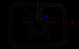
Some basic pocketing loops generated on the train today.

Using pycam's revise_directions() function it is possible to clean up the DXF data and classify polygons into pockets and islands.

There's a new parameter N_offsets

  • N_offsets=1 generates just a single offset at a specified offset-distance.
  • N_offsets=2... generates the specified number of offsets. Possibly with an increment in offset-distance that is not equal to the initial offset-distance. This happens e.g. when we want the final pass of the tool to be one cutter-radius from the input geometry but the material is difficult to machine and we want the "step-over" for interior offset-loops to be less than the cutter-radius.
  • N_offsets=-1 produces a complete interior pocketing path. Offsets are first generated at the initial offset distance and successive offsets are then generated at increasing offset distance until no offset-output is generated.

Todo: Nesting, Linking, Optimization.

There's no nesting among the loops here. The algorithm will have no clue in what order to machine the offset loops. A naive approach is to machine all loops at the maximum offset distance, then move one loop outwards, etc. But this is clearly not good as the tool would jump between the growing pockets during machining. Nesting information should be straightforward to extract from the voronoi diagram during offset-generation. The nested loops form a tree/graph, which we traverse in some suitable order to machine the entire pocket.

Also, there is no linking of these loops to eachother. For a machining toolpath one wants to link the offsets to each other so that the tool can be kept down in the material when we move from one offset loop to the next. A simple algorithm for linking should be straightforward, but I suspect something more involved is required to prevent overcutting with sufficiently complex input geometry.

When one has nested and linked offset paths, in general there still will remain "pen-up", "rapid traverse", "pen down" transitions. An asymmetric TSP solver could be run on this to minimize the rapid traverse distance (machining time).

Random points VD benchmark

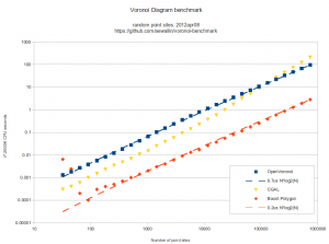
Here's some benchmark data for constructing the Voronoi diagram (or its dual, the Delaunay triangulation) for random point sites. Code for this benchmark is over here: https://github.com/aewallin/voronoi-benchmark

OpenVoronoi is my own effort using the incremental topology-oriented algorithm of Sugihara&Iri and Held. Floating-point coordinates with all sites falling within the unit-circle are used. Fast double-precision arithmetic is used for geometric predicates (e.g. "in-circle") during the incremental construction of the diagram, since the topology-oriented approach ensures that the algorithm finishes and produces an output graph regardless of errors in the geometric predicates. Quad-precision arithmetic is used for positioning vd-vertices. This benchmark runs in ca 7us*N*log2(N) time.

Boost.Polygon uses Fortune's sweepline algorithm. Only integer input coordinates are allowed, which ensures that geometric predicates can be computed exactly. Lazy arithmetic, where a high-precision slower number-type is used only when required, is used. This benchmark runs in ca 0.2us*N*log2(N) time.

CGAL uses exact geometric computation, which is slow but supposedly robust. The run-time gets worse with increasing problem-size and doesn't seem to fall on an O(N*log(N)) line.

Some thoughts:

  • OpenVoronoi is obviously too slow! Lazy arithmetic or other methods are required so that most vd-vertices can be positioned with fast double-precision code, and the quad-precision methods need to be called only rarely. OpenVoronoi uses a BGL adjacency_list to store the graph - this may also be too slow compared to a C-style "raw" data structure.
  • Other libraries which might be added to the benchmark: Triangle and QHull.
  • Held has, IIRC, reported around 0.5us*N*log2(N) for his closed-source VRONI algorithm. From the interwebs we also find this quote: "If your use is commercial, VRONI's license is a few thousand dollars."
  • It's easy to measure run-time, but how do we measure the correctness of the output that these algorithms produce? A first simple approach is write the output to a PNG or SVG file and visually inspect it, but something more precise and automated would be nice.
  • Neither Boost.Polygon nor OpenVoronoi support circular arc sites yet. Both can in principle be extended to do so.
  • Are we comparing apples to oranges? Is the output of these algorithms the same? OpenVoronoi produces a half-edge data structure of the diagram with edge-parametrizations (lines, parabolas) that allow computing a point on an edge at a given offset-distance from an adjacent site. The data structure allows for iterating through the edges, vertices, and faces of the graph.


Arc predicates

I started working on arc-sites for OpenVoronoi. The first things required are an in_region(p) predicate and an apex_point(p) function. It is best to rapidly try out and visualize things in python/VTK first, before committing to slower coding and design in c++.

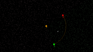
in_region(p) returns true if point p is inside the cone-of-influence of the arc site. Here the arc is defined by its start-point p1, end-point p2, center c, and a direction flag cw for indicating cw or ccw direction. This code will only work for arcs smaller than 180 degrees.

def arc_in_region(p1,p2,c,cw,p):
    if cw:
        return p.is_right(c,p1) and (not p.is_right(c,p2))
    else:
        return (not p.is_right(c,p1)) and p.is_right(c,p2)


Here randomly chosen points are shown green if they are in-region and pink if they are not.

apex_point(p) returns the closest point to p on the arc. When p is not in the cone-of-influence either the start- or end-point of the arc is returned. This is useful in OpenVoronoi for calculating the minimum distance from p to any point on the arc-site, since this is given by (p-apex_point(p)).norm().

def closer_endpoint(p1,p2,p):
    if (p1-p).norm() < (p2-p).norm():
        return p1
    else:
        return p2
 
def projection_point(p1,p2,c1,cw,p):
    if p==c1:
        return p1
    else:
        n = (p-c1)
        n.normalize()
        return c1 + (p1-c1).norm()*n
 
def apex_point(p1,p2,c1,cw,p):
    if arc_in_region(p1,p2,c1,cw,p):
        return projection_point(p1,p2,c1,cw,p)
    else:
        return closer_endpoint(p1,p2,p)


Here a line from a randomly chosen point p to its apex_point(p) has been drawn. Either the start- or end-point of the arc is the closest point to out-of-region points (pink), while a radially projected point on the arc-site is closest to in-region points (green).

The next thing required are working edge-parametrizations for the new type of voronoi-edges that will occur when we have arc-sites (arc/point, arc/line, and arc/arc).

More Medial-Axis pocket milling

My first attempt at MA-pocketing only worked when the medial axis of the pocket was a tree (a connected acyclig graph).

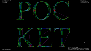
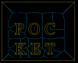
I've now extended this to work with pockets consisting of many parts which ha a MA consisting of multiple connected components. There's also simple support for when the MA has cycles, such as seen in "P" and "O" above. With a large cut-width the toolpath looks like this:

Each component of the pocket starts at the red dot with a pink spiral that clears the largest MIC of the pocket. The rest of the pocket is then "scooped out" using green cut-arcs connected with cyan (tool down) or magenta (tool up, at clearance height) rapid moves.

Instead of clearing the interior of letters we can also clear a pocket around the letters. The MA then looks like this:

This video shows quite a lot of "air-cutting". This is because the algorithm only keeps track of the previously cleared area behind the MIC that is currently being cleared. When we come to the end of a cycle in the MA the algorithm does not know that in fact MICs in front of the current MIC have already been cleared.

Medial-Axis pocketing

Update: In the US, where they are silly enough to have software-patents, there's US Patent number: 7831332, "Engagement Milling", Filing date: 29 May 2008, Issue date: 9 Nov 2010. By Inventors: Alan Diehl, Robert B. Patterson of SURFWARE, INC.

Any pocket milling strategy will have as input a step-over distance set at maybe 10 to 90% of the cutter diameter, depending on machine/material/cutter. Zigzag and offset pocketing paths mostly maintain this set step-over, but overload the cutter at sharp corners. Anyone who has tried to cnc-mill a hard material (steel) using a small cnc-mill will know about this. So we want a pocketing path that guarantees a maximum step-over value at all times. Using the medial-axis it is fairly straightforward to come up with a simple pocketing/clearing strategy that achieves this. There are probably many variations on this - the images/video below show only a simple variant I hacked together in 2-3 days.

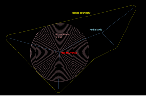
The medial-axis (MA, blue) of a pocket (yellow) carries with it a clearance-disk radius value. If we place a circle with this radius on the medial-axis, no parts of the pocket boundary will fall within the circle. If we choose a point in the middle of an MA-edge the clearance-disk will touch the polygon at two points. If we choose an MA-vertex of degree three (where three MA-edges meet), the clearance-disk will touch the pocket at three points.

MA-pocketing starts by clearing the largest clearance-disk using a spiral path (pink).

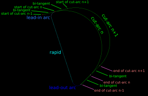
From the maximum clearance-disk we then proceed to clear the rest of the pocket by making cuts along adjacent clearance-disks. We move forward along the MA-graph by an amount that ensures that the step-over width will never be exceeded. The algorithm loops through all clearance-disks and connects the arc-cuts together with bi-tangents, lead-out-arcs, rapids, and lead-in-arcs.

This video shows how it all works (watch in HD!). Here the cutter has 10mm diameter and the step-over is 3mm.

I'll try to make a variant of this for the case where we clear all stock around a central island next. These two variants will be needed for 3D z-terrace roughing.