EMC2 tpRunCycle revisited

I started this EMC2 wiki page in 2006 when trying to understand how trajectory control is done in EMC2. Improving the trajectory controller is a topic that comes up on the EMC2 discussion list every now and then. The problem is just that almost nobody actually takes the time and effort to understand how the trajectory planner works and documents it...

A recent post on the dev-list has asked why the math I wrote down in 2006 isn't what's in the code, so here we go:

I will use the same shorthand symbols as used on the wiki page. We are at coordinate P ("progress") we want to get to T ("target") we are currently travelling at vc ("current velocity"), the next velocity suggestion we want to calculate is vs ("suggested velocity), maximum allowed acceleration is am ("max accel") and the move takes tm ("move time") to complete. The cycle-time is ts ("sampling time"). The new addition compared to my 2006 notes is that now the current velocity vc as well as the cycle time ts is taken into account.

As before, the area under the velocity curve is the distance we will travel, and that needs to be equal to the distance we have left, i.e. (T-P). (now trying new latex-plugin for math:) (EQ1)

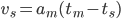
Note how the first term is the area of the red triangle and the second therm is the area of the green triangle. Now we want to calculate a new suggested velocity vs so that using the maximum deceleration our move will come to a halt at time tm, so(EQ2):


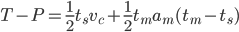
Inserting this into the first equation gives (EQ3):


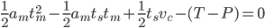
this leads to a quadratic eqation in tm (EQ4):


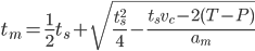
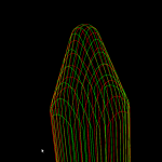
with the solution (we obviously want the plus sign)(EQ5)


which we can insert back into EQ2 to get (EQ6) (this is the new suggested max velocity. we obviously apply the accel and velocity clamps to this as noted before)


It is left as an (easy) exercise for the reader to show that this is equivalent to the code below (note how those silly programmers save memory by first using the variable discr for a distance with units of length and then on the next line using it for something else which has units of time squared):

discr = 0.5 * tc->cycle_time * tc->currentvel - (tc->target - tc->progress);
discr = 0.25 * pmSq(tc->cycle_time) - 2.0 / tc->maxaccel * discr;
newvel = maxnewvel = -0.5 * tc->maxaccel * tc->cycle_time +tc->maxaccel * pmSqrt(discr);

over and out.

Weave notes

As noted before, the waterline operation consists of radial cutter projection ("push cutter") along fibers/dexels, followed by a weave/grid construction, and contouring to produce the final toolpath. Like so:

The new Weave2 class builds up a half-edge diagram in a smart way, maintaining "next" and "previous" pointers for each edge, so that the green toolpath loop can easily be found by traversing from one CL-point to the next simply following the "next" pointer:


(The magenta arrows are "next" pointers which point from one edge to the next)

The main part of the algorithm looks at one X-fiber (from xL to xU) and one Y-fiber (from yL to yU) at a time and inserts a new internal vertex (v) into the diagram, while maintaining the existing "next" and "prev" pointers.

I didn't come up with any elegant object-oriented scheme that would do this nicely, so the build() function in the code just peeks and pokes and updates all of the 24 pointers in a brute-force kind of style.

I suspect that the O(n^2) time-complexity is optimal, since with n X-fibers and n Y-fibers there will be roughly n*ninternal vertices in the grid, and they all have to be processed (?unless we can prune the grid and ignore internal areas and focus on the edge of the weave?).

Faster Waterline

I've written a new Weave class for opencamlib which makes the waterline operation faster.

The first test-case is a single triangle, and we calculate a number of waterlines at different z-heights using a ball-cutter:

The second test-case is the Tux model where we calculate a single waterline at some z-height. Note how using the chosen ball-cutter at this particular height the waterline splits into two separate loops.

(the yellow line is a plain waterline and the red line is an adaptive Waterline, but that's not important here)

Here is the runtime data. The smaller symbols show results from the one-triangle test-case. The old algorithm(red data points and line) seems to be slower than O(N^2), with a pre-factor of about 2 milliseconds. The time data for the new algorithm (green) fits an O(N^2) line better and has an almost 10-fold faster pre-factor of around 0.25 ms.

The speedup for the Tux model (large symbols) is even greater. With the old algorithm the slope of the data points (pink) looks much worse than N^2 and runtimes quickly reach a minute or more. With the new algorithm (big light green symbols) the runtime stays under 100s even at 200 fibers/mm.

This speedup was achieved by building a weave which is a directed half-edge graph, instead of the old undirected graph. The old algorithm first used connected_components (time complexity O(V + E)) to split the weave into its connected components. For each component a planar embedding was then constructed (time complexity ??), and the toolpath loop extracted with planar_face_traversal (time complexity O(V+E)).

In the new Weave, each edge has a "next" pointer pointing to the next edge of the face. This means we can extract the toolpath loop by following the "next" pointer until we find the next CL-point. Effectively the planar embedding is now contained in the graph datastructure and does not have to be computed separately. This also saves work since we don't have to traverse faces which do not produce toolpaths. This new solution to the weave point-order problemdeserves its own post in the near future - stay tuned...

TSP

If you have lots and lots of holes to drill on your cnc-machine you might want a TSP solver to optimize the order of the holes so as to minimize rapid movements between holes. I've written a small wrapper around metric_tsp_approx from the boost graph library and included it in opencamlib as a new class TSPSolver. Here's an example on problem "u2152" from TSPLIB95.

Here's a plot of the tour length compared to the known optimal tour length, as well as the run-time on my laptop (P9400 CPU). These problems range in size from 51 points to 2103 points. I might run the bigger problems on the desktop machine later. The algorithm guarantees a tour which is at worst twice the length of the optimal tour. In practice the solutions seem to scatter around 1.4 or 1.5 times the length of the optimal tour. The run times fall neatly on the predicted O(N²*log(N) curve.

A simple greedy heuristic (with better run-time?) which always selects the closest unvisited point also guarantees a tour at most twice the length of the optimal tour.

There's also a better heuristic, the Christofides algorithm, which guarantees a tour length at most 1.5 times the optimal tour length. In addition to the minimum-spanning-tree algorithm it requires a minimum cost perfect matching algorithm. I'm not sure if there is open-source code for this somewhere.

Update: here's a run on an i7-2600K cpu. The pre-factor is now halved to about 0.2 microseconds. The largest problem has 18512 cities and takes over three minutes (217 seconds) to solve.

Here's 'usa13509' from TSPLIB. Cities with population at least 500 in the continental US. Presumably from 1995 or so.


Scaling (?)


New manual milling machine

There is a new manual milling machine in the lab, an Optimum WF-20. The design of the machine is similar to the Aciera or a Maho, with the table moving in X and Z, spindle in Y. The spindle can be flipped over for horizontal machining.

We decided to get a machine with a small work-envelope (table XY travel is 260x170 mm), but with good rigidity and hopefully good precision. The machine is around 4 keur but with the magnetic DRO and some basic accessories plus delivery the cost is closer to 6 keur. Add another 1-2 keur for toolholders and tools.

The machine has an ISO30 taper spindle with an M12 draw-bar. In addition to the 0-13mm quick-change drilling chuck in the machine there are some tools on the shelf to the right: ISO30/MT2 adapter, an ER32 chuck, 63 mm carbide-insert face-mill, another ER32 chuck, and a tapping head. There is a 150 mm rotary table on the machine to the lower left. A new 100mm precision vise is on order but not delivered yet.

This means there are now no excuses for not finishing my very delayed lathe project...

Cutter shapes

The four basic cutter shapes in opencamlib are CylCutter (cylindrical or flat-endmill), BallCutter (spherical), BullCutter (toroidal, filleted-endmill), and ConeCutter (cone, "v"-cutter).
With CompositeCutter it is then possible to combine these four into sensible combinations (such as the APT-tool). Below the combinations where the outer part of the cutter is conical, and the inner part is one of the four basic shapes. They are named CylConeCutter, BallConeCutter, BullConeCutter, and ConeConeCutter.
The general edge-push function for the cone shape isn't done yet, so there are no waterlines (except in special cases) for the cone-shape.


These inverse-tool-offset ("ITO") type images were drawn by using drop-cutter (red and green) and waterline (yellow) on a very narrow and tall triangle, so the toolpath shape looks like the inverted cutter.

Waterline fix

In the general edge-push function there was a guard against horizontal edges, since they are supposed to be handled by a special horizontalEdgePush() function. But there was no check for vertical edges. They are special too, and caused the rather strange looking behavior with BallCutter seen below.

waterline_ballcutter_error

With BullCutter the code stopped at an assert() and there was no toolpath output at all.

This is now hopefully fixed and we simply give up and return in generalEdgePush() if we encounter a horizontal or a vertical edge. These should be handled upstream by simpler specialized functions. Never assume general position is the take home message I guess...

VD algorithm animation

Some notes on the Sugihara&Iri 1994 topology-based algorithm for incremental construction of the voronoi diagram for point sites.

(A) We start with initial VD for point sites that have already been inserted. We want to insert a new site, shown as a yellow sphere.

(B) We then find the VD face to which the new vertex belongs. Among the vertices that bound this face we search for a seed-vertex, shown in pink. This is the vertex that is closest to the new generator.

(C) From the seed vertex, we search for more vertices that should be deleted(red). The vertices should form a tree (a connected, acyclic graph). Vertices that are closer to the new site than to any other site should be deleted. However due to floating-point errors it's not possible to blindly rely on an inCircle() predicate for finding the delete-tree. It's necessary to also enforce the correct topology, namely (i) the delete-vertices should form a tree, and (ii) for any incident face, the delete-vertices are connected. This ensures that no old face of the graph is deleted or split in two.

(D) Identify the edges to be deleted (red), and edges on which we need to generate new vertices (green).

(E) Generate new vertices on the green edges, and connect all the new vertices by new edges. These new edges form a new face corresponding to the newly inserted site.

(F) Remove the red/delete-vertices and edges. We are left with what we want: the VD of all the old sites and the new site.

Another picture from the original 1994 paper. The new site is not shown, but by some process we have found the delete-tree (u1,u2,u3,u4) shown as solid dots. New vertices are then generated on the "in-out" edges (u2-u10, u2-u5, u3-u6, u3-u7, u4-u8, u4-u9), shown as unfilled dots. The unfilled dots are connected with new edges (dashed lines) that form the new facet (shaded area). Image borrowed from: Sugihara&Iri 1994.

Here is an animation of the algorithm at work when inserting about 100 random points: