A roadtrip closer to home, around the archipelago route(http://www.archipelagoroute.com) Pargas-Nagu-Korpo-Houtskär-Iniö-Gustavs by car/ferry.
Text/links/images to follow, for now pics from days 1-2 are on picasa:
http://picasaweb.google.com/anders.e.e.wallin/ArchipelagoRoute2010August#
Links - 2010 Aug 5
- Narrowband Ha Filter Comparison -
- Equatorial Mounts For Budget Astrophotography? -
- Toothpick orbital sculpures -
- Asics Gel-1150 Men’s Running Shoe Review -
- Novo Blog - check out Fred Schmidt's new radio yacht design blog: http://iomdesign.wordpress.com/
- Time-lapse video of an ant colony inside of a scanner -
The weave point-order problem
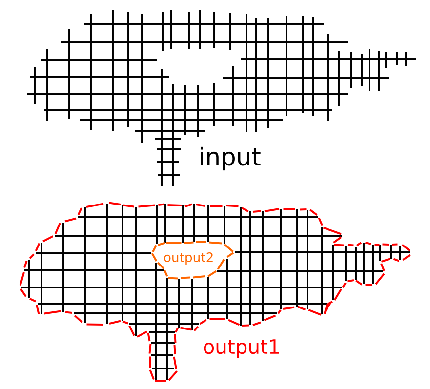
When creating waterlines or 2D offsets using a "sampling" or "CL-point based" approach the result is a grid or weave such as that shown in black above. The black lines can in principle be unevenly spaced, and don't necessarily have to be aligned with the X/Y-axis. The desired output of the operation is shown in red/orage, i.e. a loop around/inside this weave/grid, which connects all the "loose ends" of the graph.
My first approach was to start at any CL-vertex and do a breadth_first_search from there to find the closest neighboring vertices. If there are many candidates equally close you then need to decide where to jump forward, and do the next breadth_first_search. This is not very efficient, since breadth_first_search runs a lot of times (you could stop the search at a depth or 5-6 to make it faster).
The other idea I had was some kind of 'surface tension', or edge removal/relaxation where you would start at an arbitrary point deep inside the black portion of the graph and work your way to the outside as far as possible to find the output. I haven't implemented this so I'm not sure if it will work.
What's the best/fastest way of finding the output? Comments ?!
Update: I am now solving this by first creating a planar embedding of the graph and then running planar_face_traversal with a visitor that records in which order the CL-points were visited. The initial results look good:
Faster waterlines with OpenMP
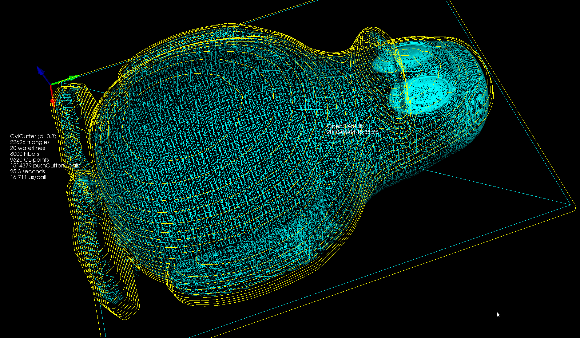
This example has three times more fibers, and thus also CL-points, than the original one, but it still runs in a reasonable time of ~15s because (1) I hard-coded the matrix-determinant expressions everywhere instead of relying on a slow general purpose function and (2) the batch-processing of the fibers now uses OpenMP in order to put all those multi-cores to work.
(red=vertex contacts, green=facet contacts, blue=edge contacts)
My initial point-ordering scheme based on a complete breadth-first-search at each CL-point is a bit naive and slow (that's not included in the 15s time), so that still needs more work.

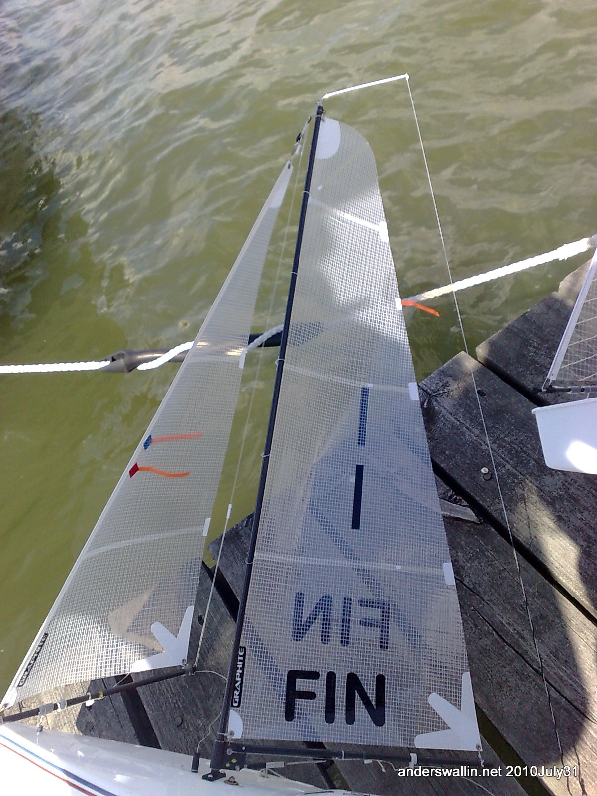
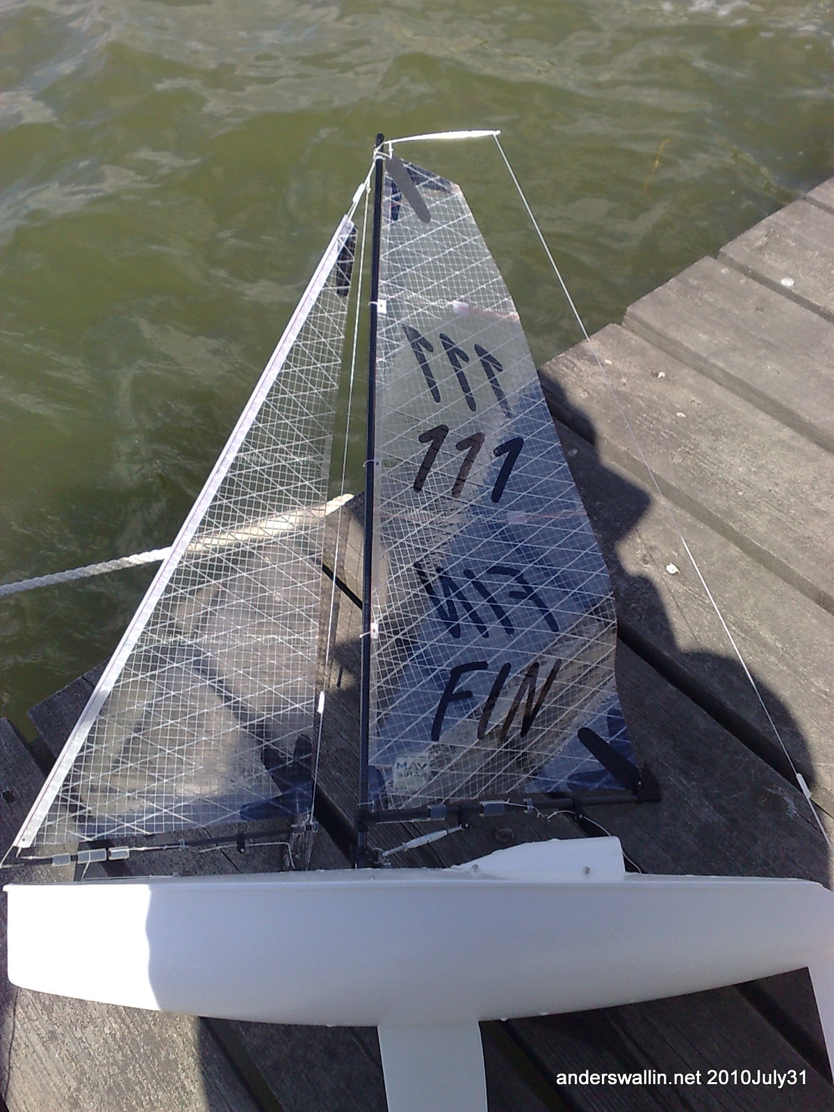
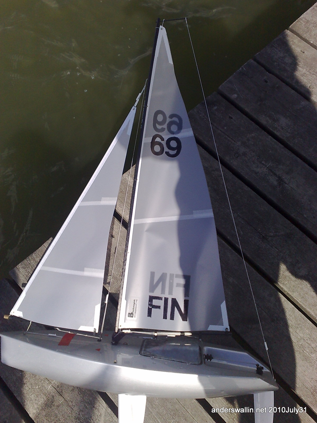
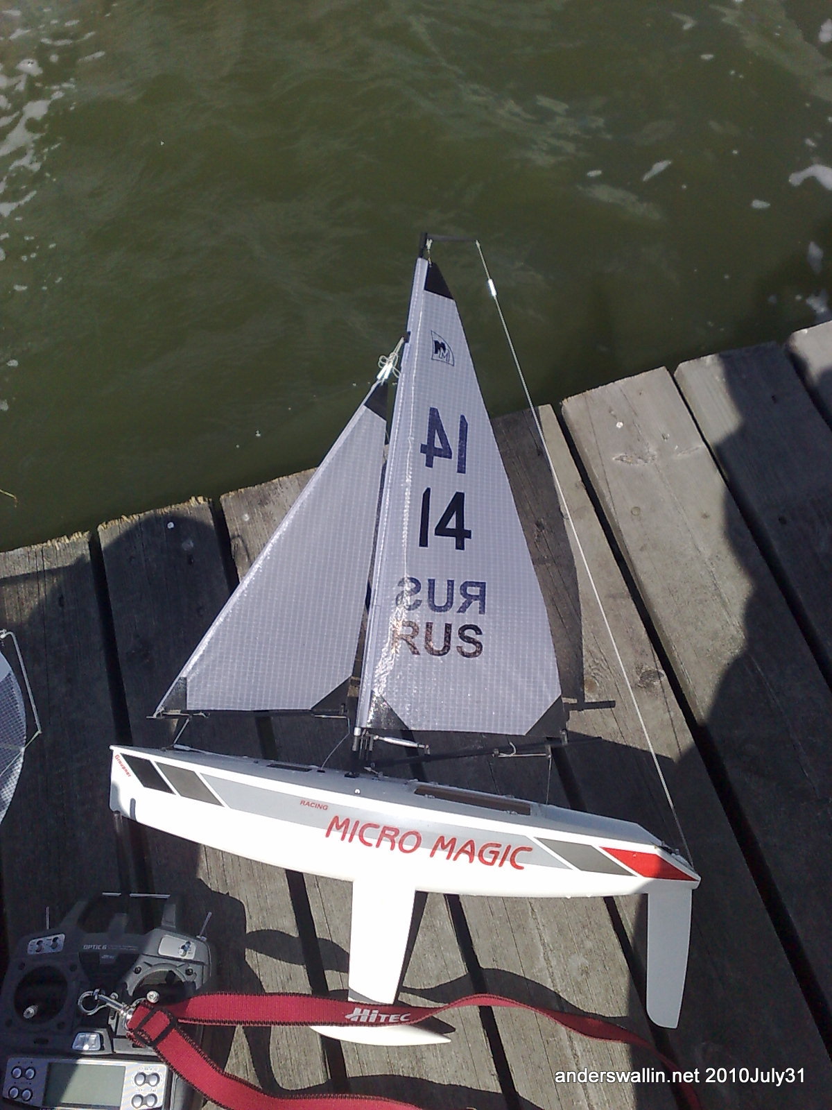
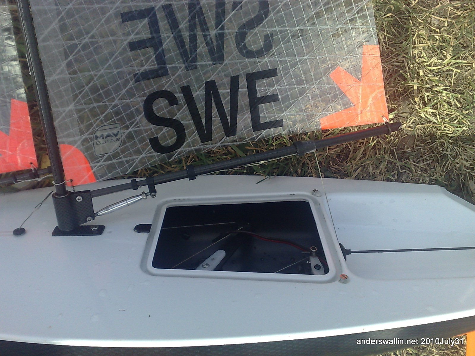
2010 Finnish MicroMagic Open
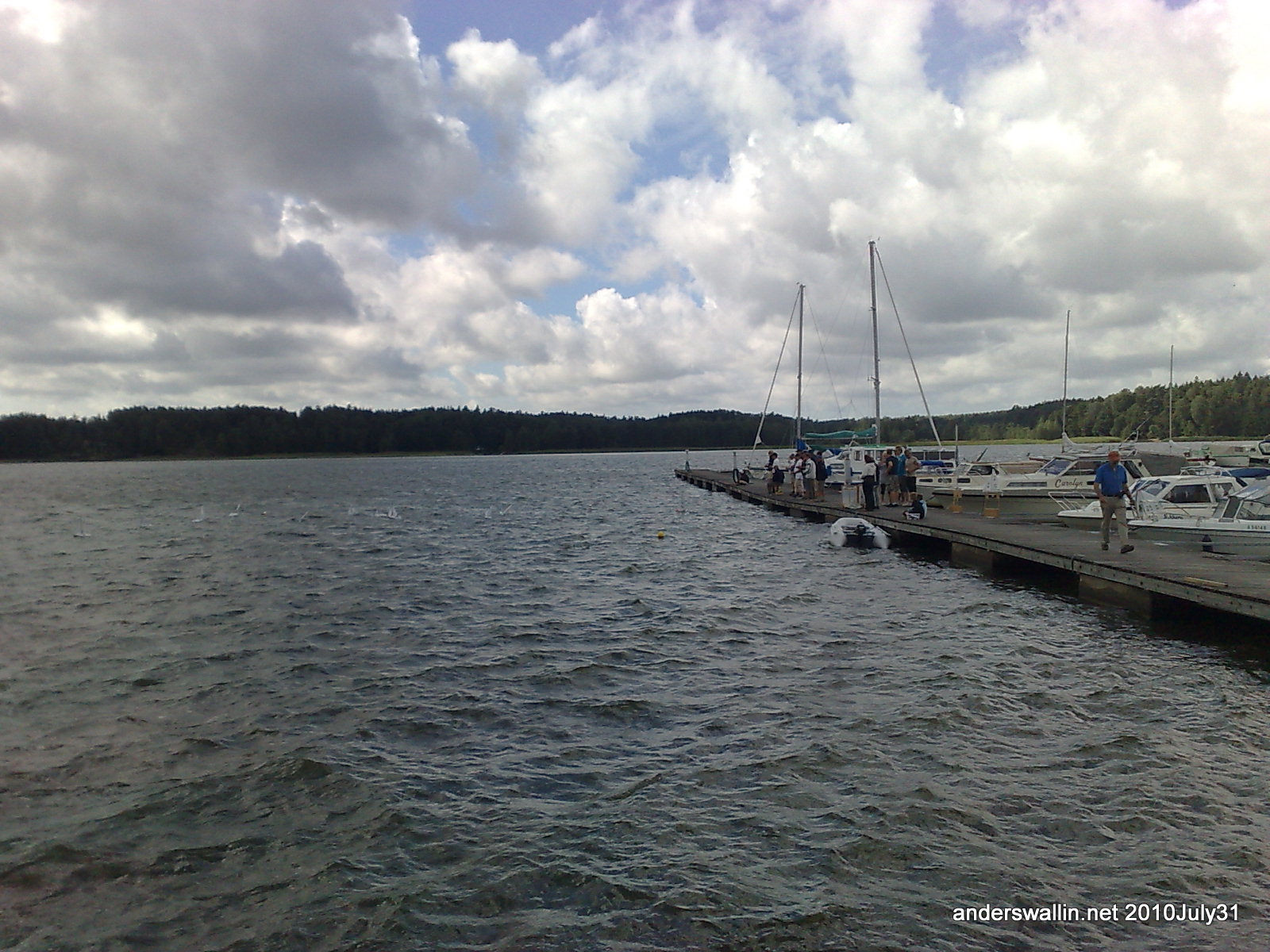
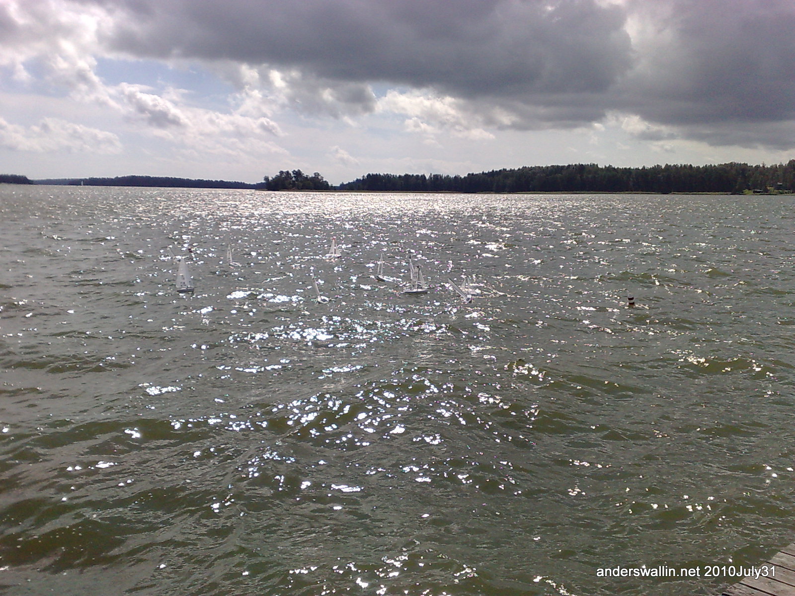
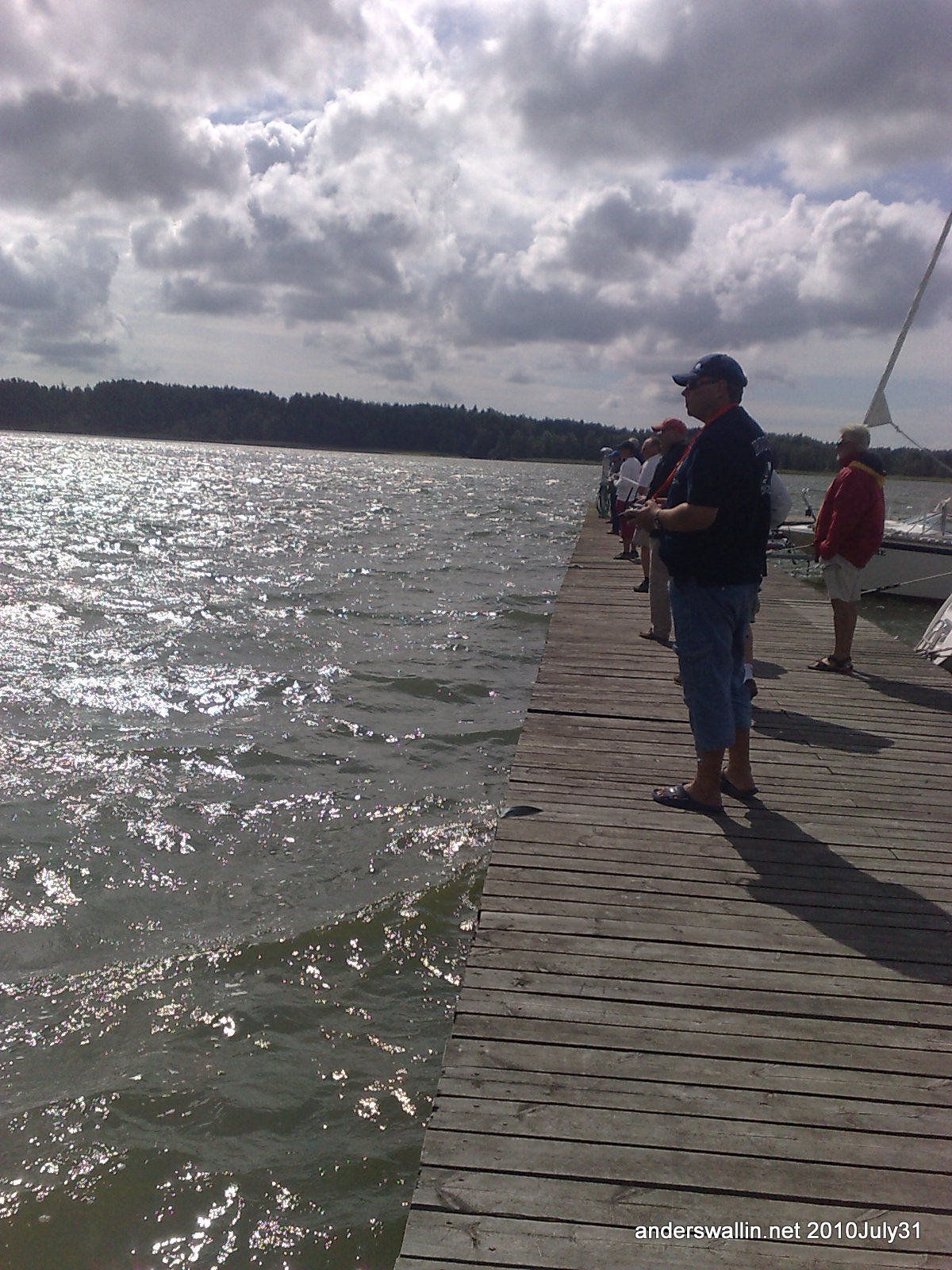
22 skippers with guests from RUS, SWE, and NED, in addition to FIN skippers came to this two-day event in Espoo. For me it was a non-event since I don't own the smaller MicroMagic rigs that were required during the first day with steady 7-8m/s and up to 11-12m/s of wind in the gusts.
At times you hear voices out there who mutter that the IOM sort of "fails" as a one-design because there isn't a minimum fin thickness, and the minimum weight is so low it is really difficult to DIY build a competitive boat on your own kitchen table. In contrast, the MicroMagic seems to do a reasonably good job of "pure one-design" with the hull and appendages, although people do play around with combinations of MkI and MkII fins and rudders.
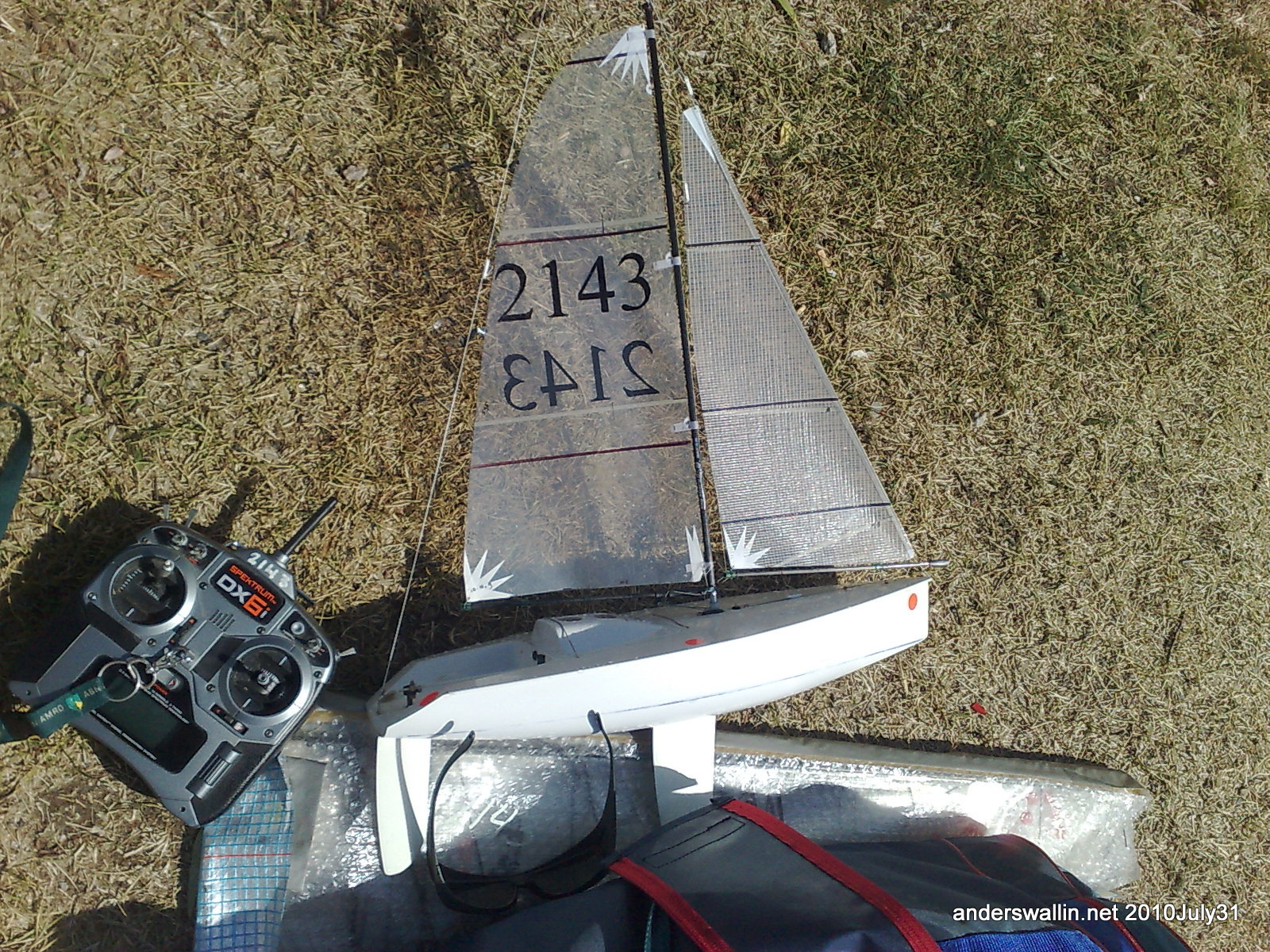
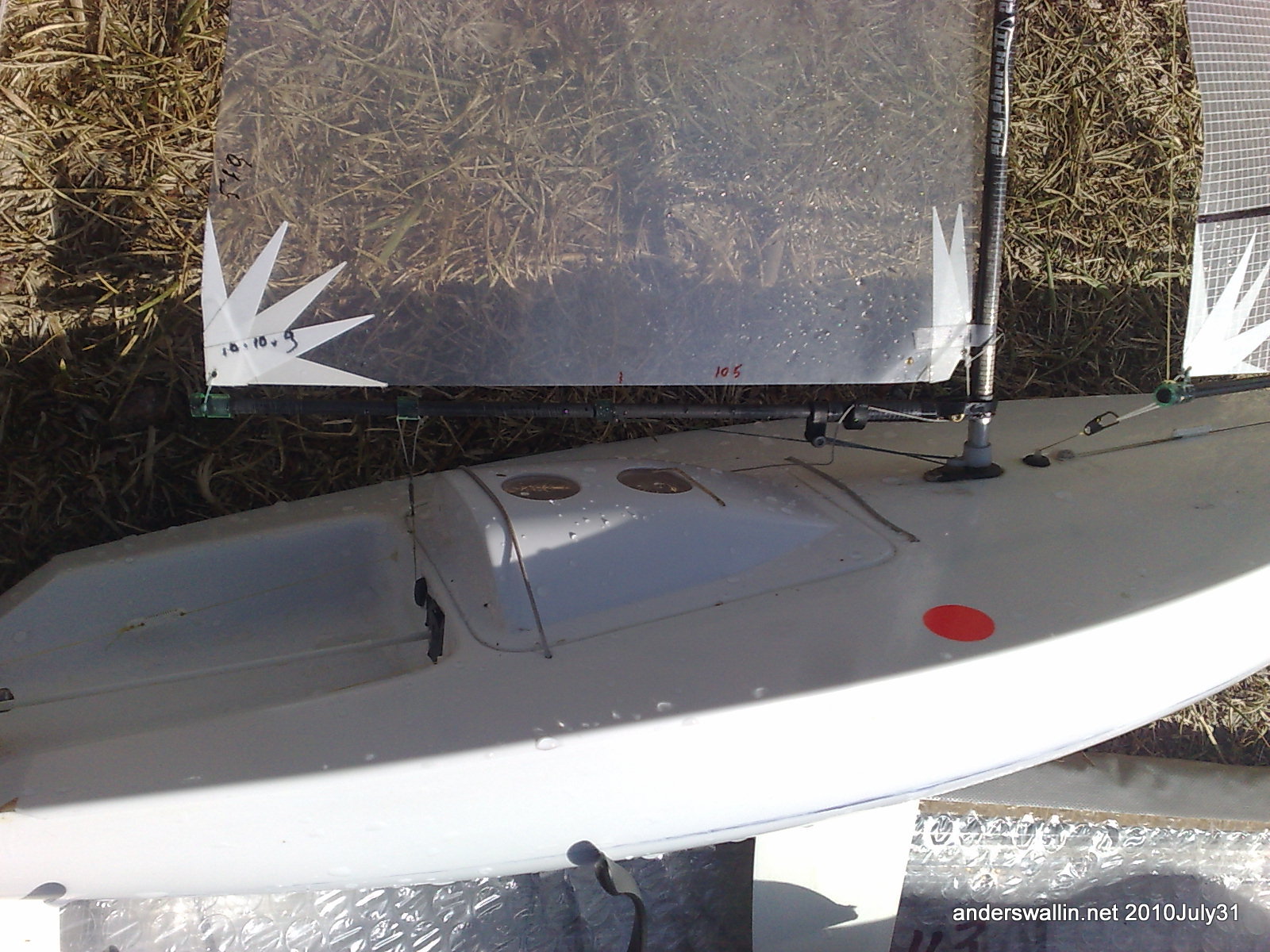
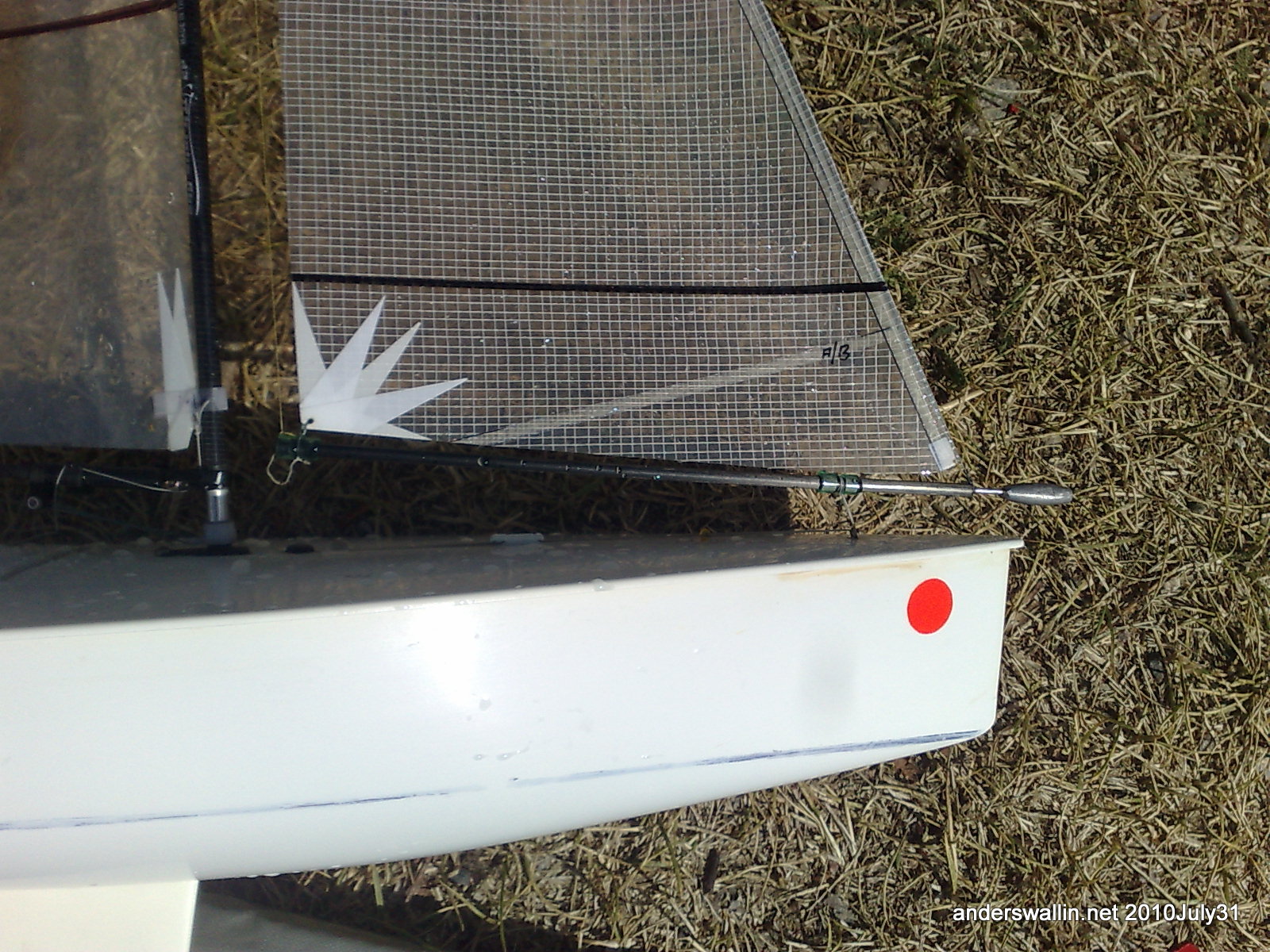
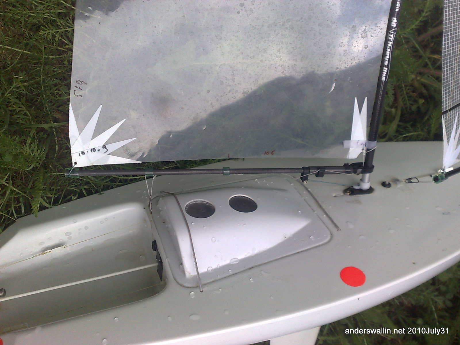
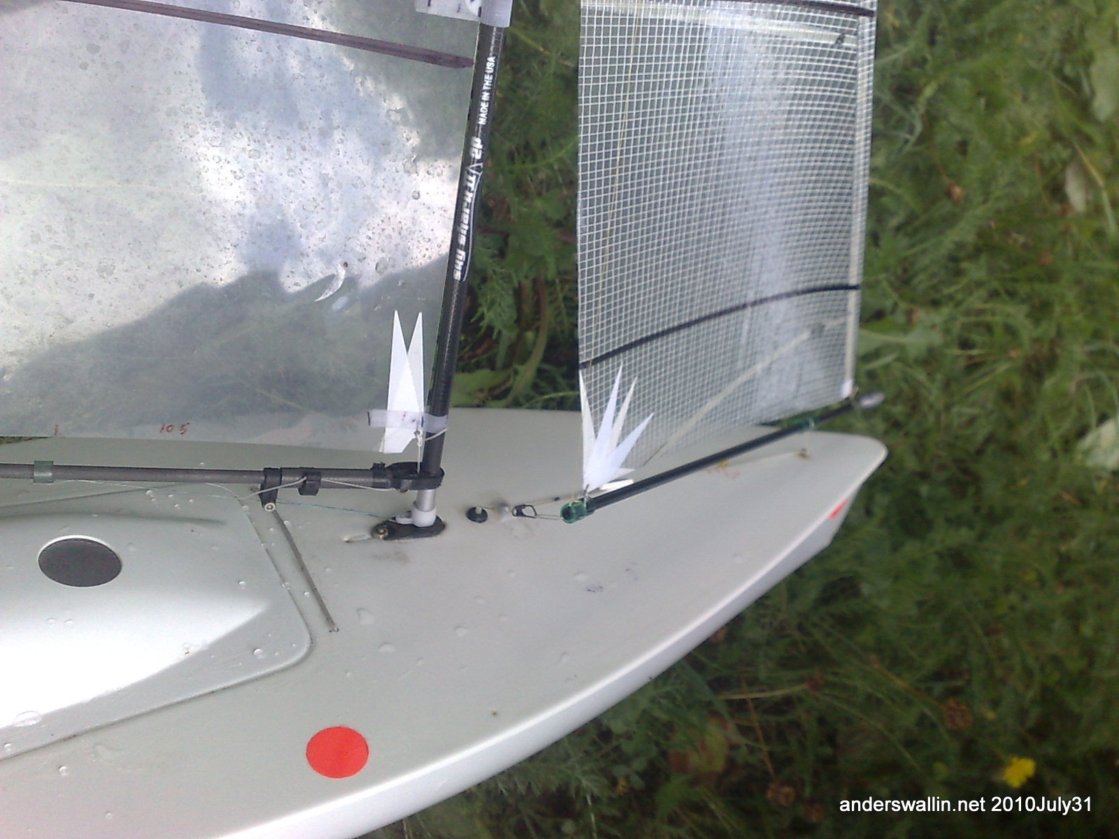
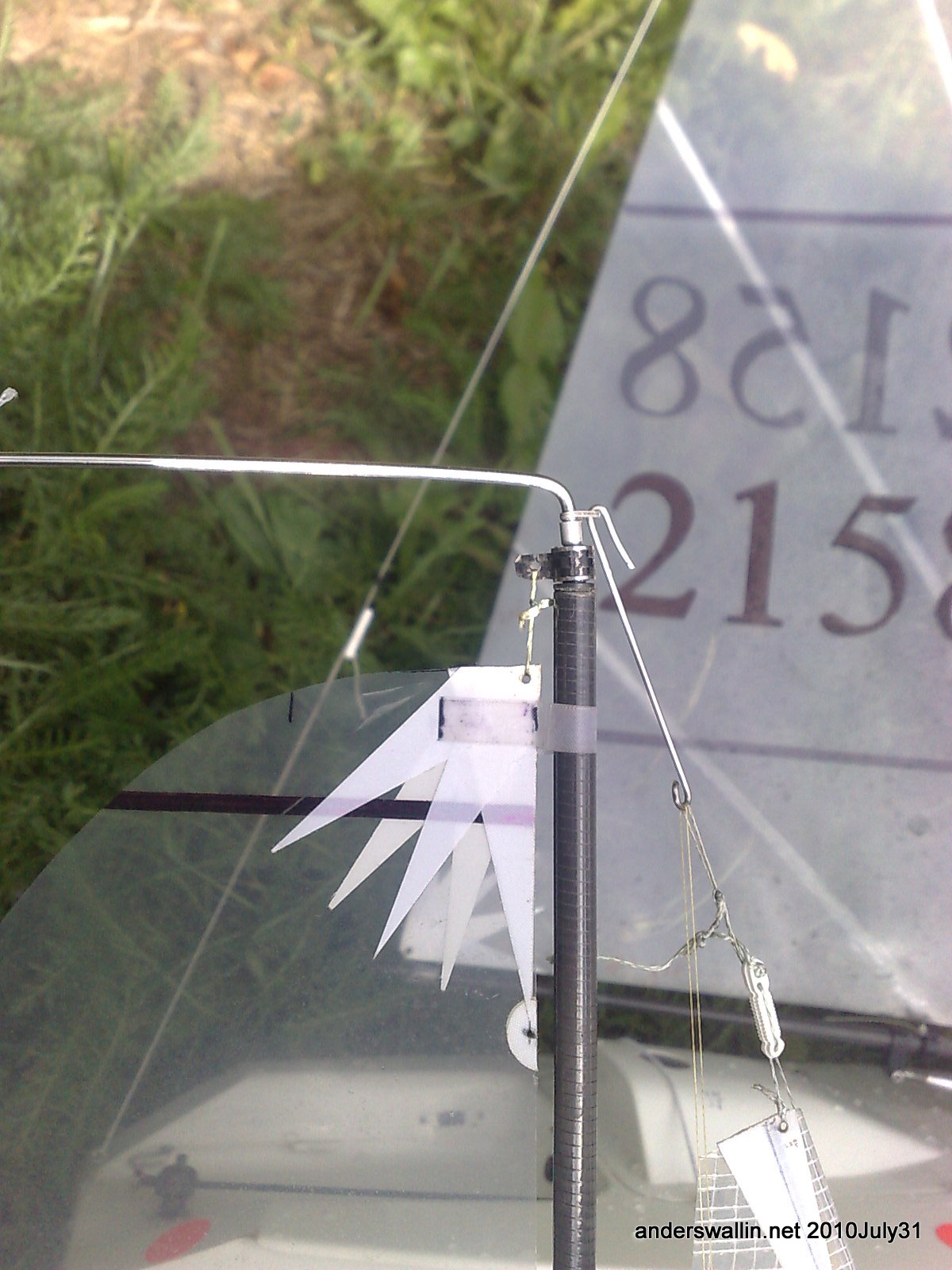
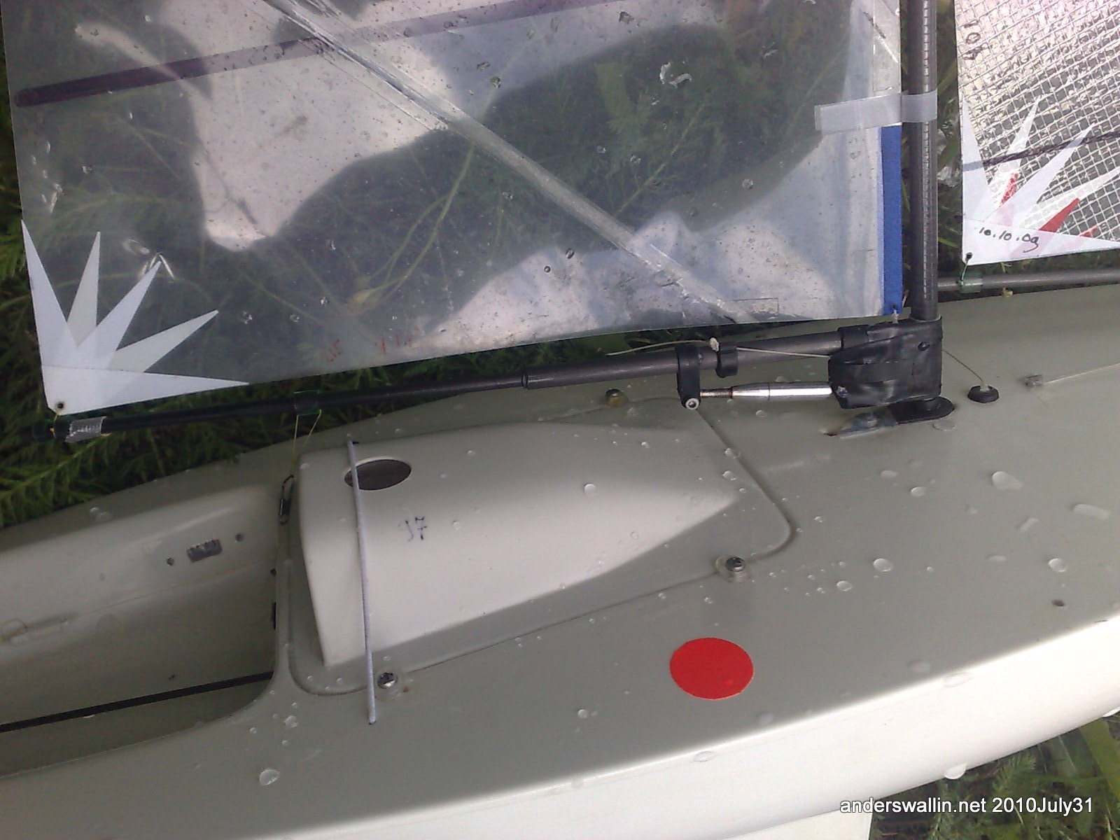
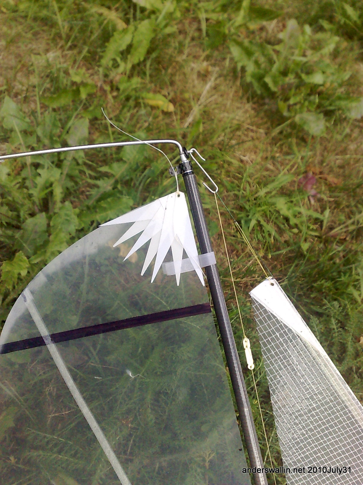
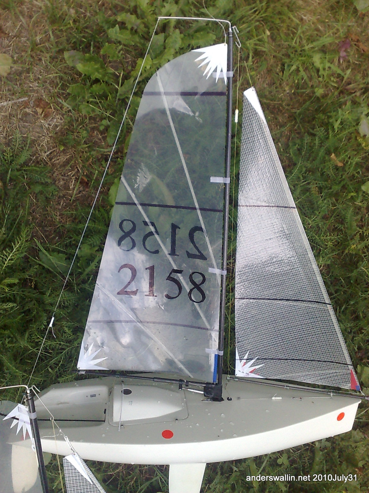
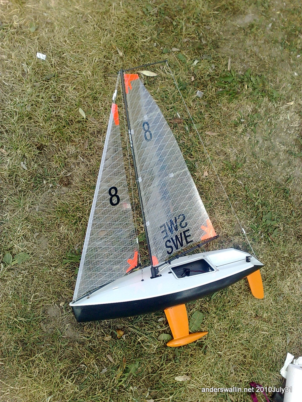
But compared to the IOM, the MicroMagic rigs are a completely wild jungle! Although the biggest no1 (or should we call it "A"?) rig is limited to the stock size sails which come with the kit, there are little or no limitations on the smaller rigs. When there is this much freedom, people are bound to explore the design envelope, and unlike a pure one-design where everyone has the same equipment it will take some experience, time, and money to converge on rig designs for the smaller sails which are competitive. People seemed to use either no2 or no3 rigs yesterday, and I photographed some of them below. The top NED and SWE boats led the field along with FIN-111 who had obviously invested in the right kind of carbon-sticks, ball-bearing thingys, and sails. It looks like it is advantageous to get both the main and jib booms as close to the deck as possible.
All of this leads to a slight illusion then when you gladly advise the newcomer that the class is cheap and uncomplicated, "you get the kit for 170eur and you are done", when in fact the competitive people swap out fins and rudders right away, and spend 4-500 euros on a set of the latest carbon-ballbearing-super-mainsail-roach-rigs. Anyone with more experience in the MicroMagic class care to comment?
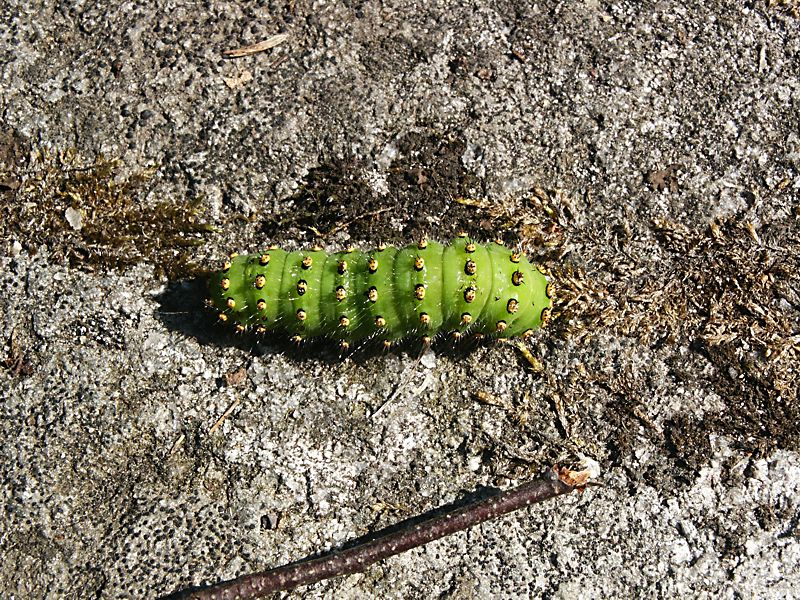
Saturnia pavonia
This swedish wikipedia page has images of the metamorphosis from egg to young caterpillar, mature caterpillar, and finally moth.
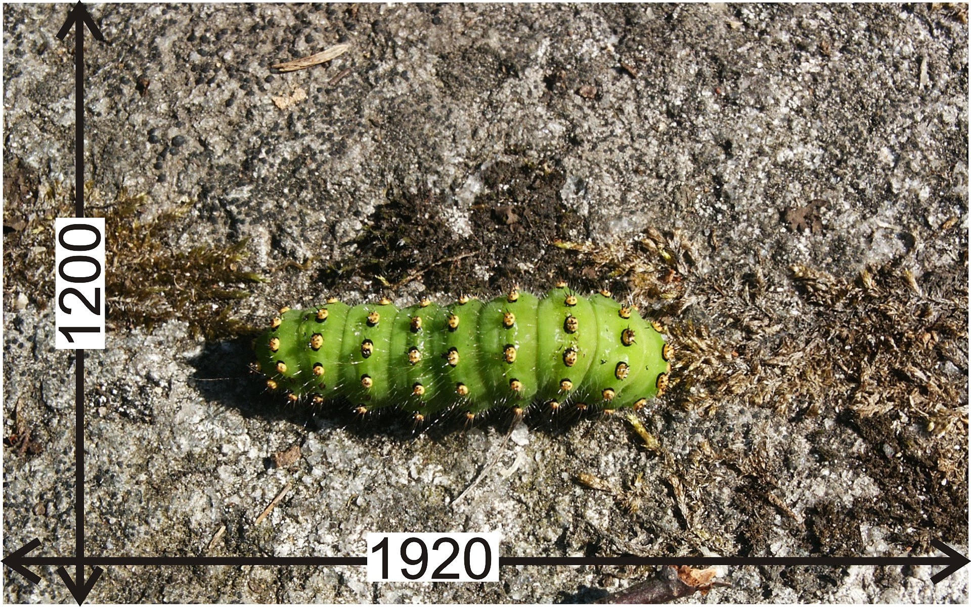
This is a bad mobile-phone photo (where are my two DSLRs when I need them!), but there's a nicer one from 2005 here (or try a big 1920 pixels wide image).

Waterline toolpaths, part 3
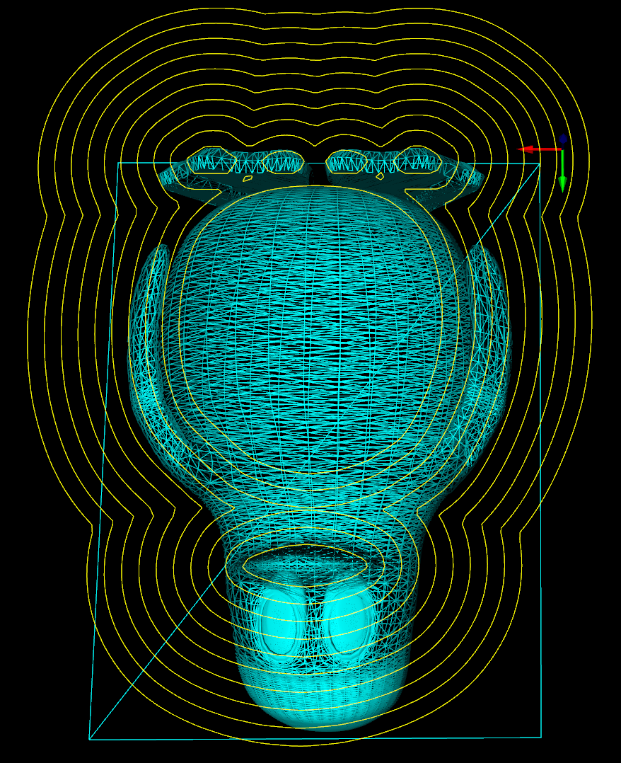
I've written a function that looks at the weave and produces a boost adjacency-list graph of it. The graph can then be split up into separate disconnected components using connected_components. To illustrate this, the second highest waterline in the picture below has six disconnected components: around the beak, belly, and toes(4). When we know we are dealing with one connected component we pick a starting point at random. I'm then using breadth_first_search from this starting point to find the distance, along the graph, from this starting CL-point to all other CL-points. We choose the point with the minimum distance (along the graph) as the next point. Sometimes many points have the same distance from the source vertex and another way of choosing between them is required (I'm now picking the one which is closest in 2D distance to the source, but this may not be correct). We then mark the newly found CL-point "done", and proceed with another breadth_first_search with this vertex as the source. That means that the graph-search runs N times if we have N CL-points, which is not very efficient...
So, compared to previously, we now have for each waterline a list-of-lists where each sub-list is a loop, or an ordered list of CL-points. The yellow lines connect adjacent CL-points.
There's still a donut-case, where one connected component of the weave produces more than one loop, which the code doesn't handle correctly.
Links - 2010 Jul 29
- Voronoi mapping makes pretty, efficient circuit boards -
- DIY powder coating rig -
- C02 laser in your living room -
- Fishing Lure Syndrome -
- Canon EOS Best lens list updated -
- Truetype Tracer 4.0 is released -
- Micro mill from scrap aluminum -
- Incredible 35 minute video tour of the ISS -
- Constant cusp toolpath generation in configuration space based on offset curves -
- Direct slicing of cloud data with guaranteed topology for rapid prototyping -
Jakob halvmaraton 1:50:37
This week the plan was to do the last 20+ km run before the Helsinki marathon, which is in three weeks on 14 Aug 2010. But since I was in the region and there was a race, I did the Jakob half-marathon instead. Results and info at http://jakob-marathon.net/
This is a small event with 4-500 runners, so less walking, pushing, and passing in the beginning than at HCR or Forssa. I didn't really set a time-goal, just ran in the beginning at a pace that felt right, which today was around 5:11 to 5:20/km. There were four drinking stations at a little after 4, 8, 12, and 16 km which show up as slightly slower kilometers in the data. Towards the end a few faster kilometers would have maybe allowed a sub 1:50 time.
The grey background shows roughly the level of detail which google earth/maps provides in this part of the country...

"He de maraton e noo flaka beta!"
By popular demand, an openstreetmap rendering. Fiddled around with the openstreetmap.org website but could not get it to display my GPS trace on top of the map. When searching for "gps" ubuntu suggests tangoGPS, but that doesn't reder gpx-traces either. Then downloaded and installed Merkaartor, which does show gpx-traces after clicking around for a bit to learn how it works. At a zoom level which shows the whole route Merkaartor doesn't show individual streets, so I zoomed in a bit, exported two bitmaps (top/bottom) from Merkaartor, and manually stitched them together in GIMP.
