
Long time no run. These slow 10+ k jogs need to happen every week now if the HCR half-marathon, to which someone at work challenged a lot of people, is going to happen.
Long time no run. These slow 10+ k jogs need to happen every week now if the HCR half-marathon, to which someone at work challenged a lot of people, is going to happen.
explanation(s) to follow at some point...
Recursion and 'divide-and-conquer' must be two of the greatest ideas ever in computer science.
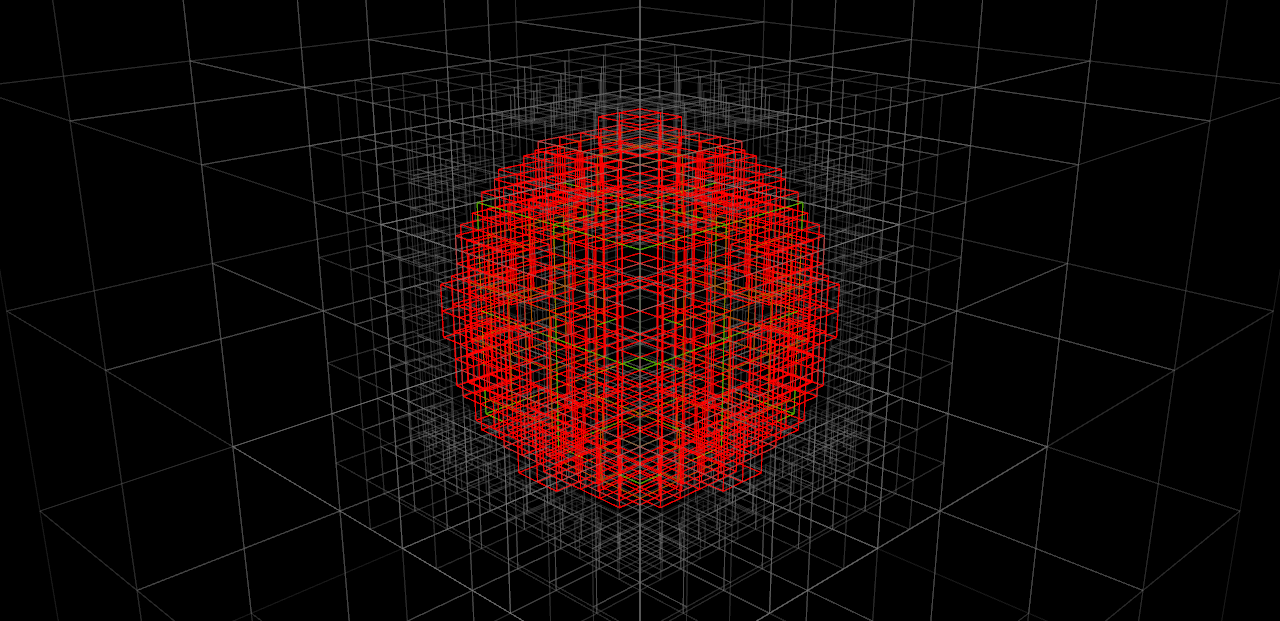
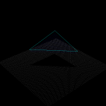
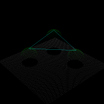
Threw together some code in python today for building an octree, given a function isInside() which the tree-builder evaluates to see if a node is inside or outside of the object. Nodes completely outside the interesting volume(here a sphere, for simplicity) are rendered grey. Nodes completely inside the object are coloured, green for low tree-depth, and red for high. Where the algorithm can't decide if the node is inside or outside we subdivide (until we reach a decision, or the maximum tree depth).
In the end our sphere-approximation looks something like this:
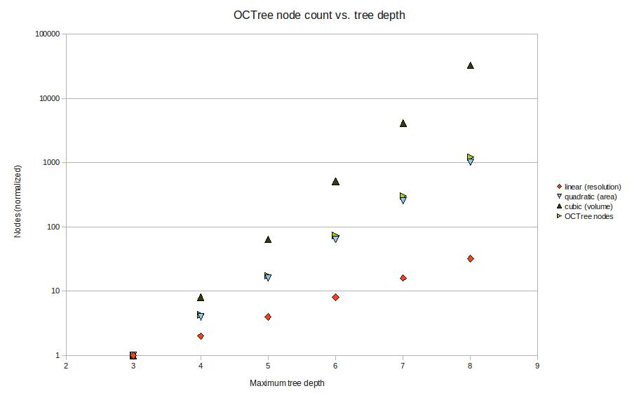
These tests were done with a maximum tree depth of 6 or 7. If we imagine we want a 100 mm long part represented with 0.01 mm precision we will need about depth 14, or a subdivision into 16384 parts. That's impractical to render right now, but seems doable. In terms of memory-use, the octree is much better than a voxel-representation where space is uniformly subdivided into tiny voxels. The graph below shows how the number of nodes grows with tree-depth in the actual octree, versus a voxel-model (i.e. a complete octree). For large tree-depths there are orders-of-magnitude differences, and the octree only uses a number of nodes roughly proportional to the surface area of the part.
Now, the next trick is to implement union (addition) and difference (subtraction) operations for octrees. Then you represent your stock material with one octree, and the tool-swept-volume of your machining operation with another octree -> lo and behold we have a cutting-simulator!

In colours and numbers, the number of iterations in the offset-ellipse solver required to reach an arbitrary 8-digit precision. A smart choice of initial value can save almost half of the computation.
Jari has been making eyebolts in brass and stainless steel with the cnc mill. These are M3 bolts with a hole/eye on the end. They are bolted to the deck of model yachts and provide attachment points for the jib, shrouds, and backstay.

More on the offset-ellipse calculation, which is related to contacting toroidal cutters against edges(lines). An ellipse aligned with the x- and y-axes, with axes a and b can be given in parametric form as (a*cos(theta) , b*sin(theta) ). The ellipse is shown as the dotted oval, in four different colours.
Now the sin() and cos() are a bit expensive the calculate every time you are running this algorithm, so we replace them with parameters (s,t) which are both in [-1,1] and constrain them so s^2 + t^2 = 1, i.e. s = cos(theta) and t=sin(theta). Points on the ellipse are calculated as (a*s, b*t).
Now we need a way of moving around our ellipse to find the one point we are seeking. At point (s,t) on the ellipse, for example the point with the red sphere in the picture, the tangent(shown as a cyan line) to the ellipse will be given by (-a*t, b*s). Instead of worrying about different quadrants in the (s,t) plane, and how the signs of s and t vary, I thought it would be simplest always to take a step in the direction of the tangent. That seems to work quite well, we update s (or t) with a new value according to the tangent, and then t (or s) is calculated from s^2+t^2=1, keeping the sign of t (or s) the same as it was before.
Now for the Newton-Rhapson search we also need a measure of the error, which in this case is the difference in the y-coordinate of the offset-ellipse point (shown as the green small sphere, and obviously calculated as the ellipse-point plus the offset-radius times a normal vector) and where we want that point. Then we just run the algorithm, always stepping either in the positive or negative direction of the tangent along the ellipse, until we reach the required precision (or max number of iterations).
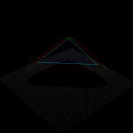
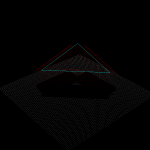
Here's an animation which first shows moving around the ellipse, and then at the end a slowed-down Newton-Rhapson search which in reality converges to better than 8 decimal-places in just seven (7) iterations, but as the animation is slowed down it takes about 60-frames in the movie.
I wonder if all this should be done in Python for the general case too, where the axes of the ellipse are not parallel to the x- and y-axes, before embarking on the c++ version?

Contacting a toroidal cutter (not shown) against an edge (cyan line), is equivalent to dropping down a cylindrical cutter (lower edge shown as yellow circle) against a cylinder (yellow tube) around the edge, with a radius equal to the tube-radius of the original toroidal cutter.
The plane of the tip of the cylindrical cutter slices through the yellow tube and produces an ellipse (inner green and red points). The way this example was rotated it is obvious where the center of the ellipse along the Y-coordinate (along the green arrow) should lie. But the X-coordinate (along the red arrow) is unknown. One way of finding out is to realise that the center of the original toroidal cutter (white point) must lie on an offset-ellipse (outer green/red points). Once the X and Y coordinates are known it is fairly straightforward to find out the cutter-contact point between the cylindrical cutter and the tube, and from that the cutter-contact point between the toroid and the edge. Finally from that the cutter-location can be found.
Something to implement in opencamlib soon...
For spherical cutters (a.k.a. ball-nose), the vertex-test (green dots), and the facet-test (blue dots), are fairly trivial. The edge-test (red-dots) is slightly more involved. Here, unlike before, I tried doing it without too many calls to "expensive" functions like sin(), cos() and sqrt(). The final result of taking the maximum of all tests is shown in the "all" image which shows cutter-locations colour-coded based on the type of cutter-contact.
The logical next step is the toroidal, or bull-nose cutter. Again the edge-test is the most difficult, and I never really understood where the geometry of the offset-ellipse shows up... anyone care to explain?