8h Rogaining, Espoo

Took part in an 8h rogaining event yesterday. Very wet in the forest with a lot of fallen trees due to the storms over the last few weeks.

We planned a ca. 20km long route (straight lines between controls), assuming we would walk up to 50% more, i.e. around 30km, which would be OK for 8 hours.

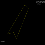
This event had a 1:25000 map which was much easier to read compared to the 1:40000 one last fall. No problems in the beginning, we fould 23 -> 21 -> 31 -> 41 quite easily. The first digit of the control-numnber indicates how many points you get for the control. The next control 51 was worth five points, and they are usually harder to find. Not this time, since it was at the very top of a hill, and people before us had already left tracks in the snow.

Then comes the big mistake of the day. We follow another faster group west down the hill from 51 towards 32. For some inexplicable reason we then completely mis-place ourselves on the map and although we are practically within reach of 32 we make a slow detour south before we realize where we are. Update: I have since learned that our confusion most probably was caused by a brand new road in this area, which was not marked on the map!

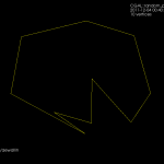
Probably annoyed by the first mistake, the second mistake of the day comes on the very next control: between 32 and 37 we take the wrong path north-east and decide to head back when we realize that.

So far we had stuck to the plan, but looking at the watch at 37 we decided to cut 39 from the route. Walk north along the road to 26, and then more walking along a big and then a small road to 57. At 57 we had some discussion about whether to walk back along the road, or try to find the electric lines north of 57 and let them guide us to the road. We had used 4 hours, or half of the total time here. We chose the latter route, and a straight northward pointing bit of our path after 57 indicates where we walked under the electric lines. Close to 53 the plan was to follow a path to the right of the hill and then the ditch to the control. Things didn't go to plan and we ended up to the left of the hill, but found the control with the help of tracks in the snow and voices/lights of others. A walk along the lake-shore to 55. And further north to a road.

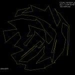
So far we had roughly followed the plan. But now we had less than 3 hours left, and it was already dark making orienteering in the woods without clear paths or roads much harder. We decided to forget the plan and walk mostly along roads towards the finish, taking controls close to roads/paths along the way. A long bit of walking first south and then northeast to 49. Another long bit of walking all the way to 24. Here the image shows double GPS-paths because I switched from the 405cx watch to the Edge800 I use on the bike. We still had 45-50 minutes left at 24, so with a close eye on the clock we find 33 quite easily and 22 with a little more effort. We finished with about 12 minutes to spare.

About 90 teams (either solo, or in teams of 2-4 persons) took part.

Update, here's our route again (in red), compared to another slightly faster team's route in blue:

Update 2: map with tracks from three teams:

TTT++ and font-vd

Update: Now all the capital letters work!

I wanted to test my VD algorithm on font-outlines. So I ported Chris Radek's truetype-tracer to c++ and added some python bindings. Here: https://github.com/aewallin/truetype-tracer

Because my VD code cannot handle circular arcs yet, I took some old code from TTT 3.0 and made converting conics and cubics, the native output of FreeType, as well as arcs into line-segments optional.

Predictably, OpenVoronoi crashes in many cases, but here is an "L" that works:

VD for polylines and polygons

I've been hacking away at openvoronoi, adding support for polylines and polygons.

The code I had in November works with individual non-intersecting line segments, like this:

Note how each vertex in the figure above is of degree three, i.e. there are three edges incident on each vertex. There's something about the number three, or triangles, or both, that makes planar graphs of degree three particularly nice to work with.

Here's the same figure with some notes describing the elements. The line-sites are drawn in yellow, and are associated with their left R(L+) and right R(L-) regions. The purple lines are called separators, and they define the region associated with the start- or end-point of a line-site. The three possible edge-types are also shown: LineEdge between two point-sites, LineEdge between two line-sites, and a Parabolic (PointLine) edge between a point-site and a line-site.

Now, things get more complicated when we want to 'glue' two line-segments end-to-end in a polyline, or glue three or more line-segments together to form a polygon. Vertices are not necessarily of degree three any more. In fact the vertex degree is essentially unbounded, as you can start/end arbitrarily many line-segments at the same vertex. The solution I am using is to introduce what I call a null-face with zero-length null-edges around each point-site to which more than one line-segment connects. The mental picture is much like that of a key-chain, or mountaineering carabiners that are hooked-in to a loop. When we want to use the a vertex as a start/end-point for a segment we 'hook-in' to the null-face:

This introduces a number of new rules and associated code for how vertices should be created, removed, and moved around a null-face, but it seems to work somehow now:

Note how these null-faces and the circular null-edges around each end-point result in degree three vertices, which are much nicer to deal with in the algorithm. For example, the null-face around vertex "0" is 40->85->86->41->39. Without the null-face construction this vertex would be of degree five. Here is an annotated version of the same picture:

This image shows how the diagram divides the plane into regions associated with endpoints such as R(0) and with the right/left side of a line-segment such as R(0-29) and R(29-0). The null-edges that form null-faces around each end-point are drawn in white.

Of course, these null-edges are only a topological construction. Geometrically we can position each vertex on a null-face at the location of the encircled point-site. This effectively contracts away the zero-area null-faces, and the result is the diagram we want:

The code now runs for a few select test-cases. To be continued...

Update: The code now seems to work also for random polygons with a large number of vertices. Here is one with 400 vertices:

and 3200-vertices:

Call graph

For profiling I made a small c++ program which calculates a poisson voronoi diagram. When called through valgrind like this (under valgrind the program will run roughly 50 times slower than normal)
valgrind --tool=callgrind -v ./ovd_tst --n 1000
I can then use kcachegrind to draw a call graph.

I thought the nearest-neighbor grid-search (grid_find_closest_face()) would cost much more than it does.

The callee map may in fact better visualize where CPU time is spent:

The map changes significantly if we change the solver number type to double, which is faster but less accurate. A better strategy might be to run the fast solver(double) first, then check the quality of the solution, and run the slow solver(qd_real) only if necessary.

In this map there doesn't seem to be an obvious bottleneck or 'hot spot' in immediate need of optimizing, since there are 6-8 blocks/functions each taking roughly 10% of the CPU time.

After some tweaking the benchmark (with the double solver) run gives these results:

Poisson Voronoi diagram statistics

On g+, John Baez linked to work by Henk Hilhorst on the probability of finding voronoi cells with n sides in a poisson voronoi diagram.

A poisson voronoi diagram has point sites randomly and uniformly distributed, like this:

Here's the distribution I came up with, after counting the edges for each voronoi cell from 200 runs where openvoronoi generated the diagram for 100k point-sites in each run. The green line is Hilhorst's prediction. I'm assuming poisson statistics, so if the bin-count for a certain n is fn, I've drawn errorbars of length sqrt(fn). Cells with n=15 or n=16 are so rare that the statistical error is of the same size as the probability (but it does agree with Hilhorst's prediction). Among the 20M cells I looked at I did not find n >= 17. For n=17 the predicted probability is 2e-9, so there's should be a 50% chance of seeing one if I would produce 500M random cells (that would take about 7 hours of CPU time).

The relevant papers are

The logarithmic y-axis hides the fact that the distribution is very peaked around n=6, so here is a plot with a linear y-axis:

Colorhug build

The other parts for a Colorhug already arrived, and we got the missing color sensor TCS3200D, from Mouser last week.

Please don't laugh at my SMD soldering skills 🙂

I made a first PCB using the original pcb-layout from the git repo, but the combination of a printer driver that produced a fuzzy mask and less than perfect etching skills didn't produce a satisfactory result. I then re-drew the GND copper-fill and some other traces on the PCB for bigger clearances and easier etching. Printed from adobe acrobat on windows the mask also has much better resolution than when printing from Document Viewer/Ubuntu.

Here are my modified masks in PDF format: hardware_etched_2011dec04 (note that the board outline is enlarged)

The PCB is clearly made for commercial production. There are vias under the microcontroller, which you can see from the pictures I have filed down after soldering so that the chip will fit on top. This isn't an issue with a commercially produced PCB where the vias are plated. Also, I noticed while starting to assemble the board that the large pad on the 3.3V regulator in the upper right corner will short out the trace drawn under it. Thus the silicone tape as insulation in the following picture. This is also not an issue with a commercial PCB since it will have an insulating soldermask.

Then on to programming. From the servodrive adventure I have an ICD2 programmer/debugger. However using it was challenging. I first tried 64-bit Windows 7. The latest Microchip MPLAB IDE does ship with 64-bit drivers, but they are hidden away in a special place, and require manual installation. No luck here, from device-manager/update-driver I couldn't get Win7 to recognize a valid driver using the instructions supplied.

I then tried 64-bit Ubuntu11.10. They have a Java version of MPLAB, called MPLAB X. It installs and runs nicely, but when I started digging in the documentation it turns out that product only supports the newer ICD3 programmer/debugger, not my older ICD2! (there might be ICD2 support in some old beta-version of MPLAB X, but I didn't search).

Oh well, it's nice we keep those old 32-bit Windows XP machines around in the lab! So I repeat for the third time the whole download and installation process on an old XP machine. That seems to work. The C-compiler which I vaguely remember being free previously now has a 60-day trial period after which Micrchip proudly proclaims it will stop producing nice binaries and start producing crap binaries. Strange. There's both a bootloader and a firmware project in the colorhug firmware repo. My guess is I only need to build and deploy the bootloader, and the firmware can be flashed from any machine after that. The bootloader requires a USB-library, which I didn't manage to find before I had to quit for the day... To be continued.

Note to self: future projects should use ATMEL or other microcontroller which (a) has a free/open-source toolchain for building the firmware, and (b) can be programmed directly over USB. The 6-pin ICSP connector is just big and ugly on a cute little board like this.

Random polygons with CGAL

At some point I'm going to need random simple polygons for testing my voronoi diagram code. CGAL includes a function random_polygon_2 which uses the "2-opt" heuristic (see Auer&Held-1996).

I wrote a minimal boost::python wrapper around this function in order to test it and draw the polygons using vtk. Here are some examples of random polygons with randomly placed vertices inside the unit circle:


The one with 8k vertices takes 150 seconds of i7-2600K CPU time to generate. The worst-case running time of this algorithm is slow, O(n^4 log n), but it practice it seems better than O(n^3):

Code: https://github.com/aewallin/randompolygon

Another Nokia N9 vs. Garmin GPS test

These results are much like my previous ones. Close to buildings or other difficult places the N9 GPS performs significantly worse than the Garmin. This is somewhat surprising since the N900 performs very similar to a Garmin. Could better GPS-data on the N9 be just a software-update away? When is someone going to try to get TJ Lindfors's RTK-GPS Openmoko hack to work on the N9 ?!