Bulbs of Steel

As a first serious test-run for our now servo-controlled cnc mill we decided to make an IOM bulb out of steel. It ends up a bit bigger in volume when made out of steel compared to lead, but the difference isn't huge. Making it with a cnc mill allows designing almost any reasonable 3D shape you can imagine.

The mill worked fine during the whole run, about 3 hours of rough-cutting and 1.5 hours of finish cutting, but there was a slight operator error in the setup which means this bulb will likely not sail. The following error stayed low throughout the run, and the servos weren't even hot to the touch after the workout.

We used adaptive roughing paths and then a simple parallel finish path. Both operations are cut with an 8 mm flat cutter. The adaptive paths did seem to work, and on this size machine they are really handy since a slight over-cut will likely stall the spindle motor (1.5 kW and 5000 rpm, small by big-iron cnc-standards).

0:00 rough cutting begins. The stock is a 45 mm diameter steel bar, face-milled down on the sides so it can be clamped to the machine vises. Note the cutting feedrate which is 500mm/min and 'high-feed' in the (x,y)-plane when the tool is positioned for the next cut. When the tool lifts up to the clearance plane it does normal G0 (rapid) moves.
1:34 more rough cutting on the other end of the bulb.
1:58 still pics of the rough-pass almost ready
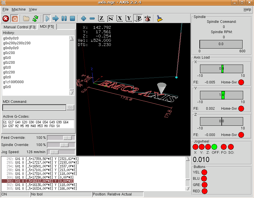
2:15 view of emc2 while cutting. Note pyVCP bar widgets showing commanded PWM to servo motors.
4:29 beginning of parallel finish cut. programmed feed 1500 mm/min which is attained briefly in the middle of the move.
5:00 more finish cutting, about 2/3 done.
5:50 another view of emc2 and the pyVCP panel. Note Y and Z motors working to position the tool. The following error for each axis is also shown.
6:15 still pictures of the finished bulb (well, one half of it anyway). Note at the front of the bulb we tried to run the program at 150% of programmed feedrate, but that didn't work at all and resulted in a poor surface finish. We did try to slow down also from 100% but that didn't improve the surface much.

Google video doesn't really do justice to the nice 640x480 video and 5 Mpix still-photos that come out of the N95, so if you've bothered to read this far, here's the original 100 Mb mp4 (I hope I don't exceed my bandwidth limit).

Helsinki Model Expo 2008

Model Expo along with cats, dogs, snakes, and Llamas at PetExpo, and everything family-ish you can imagine at Child'08 happened over this weekend at the Helsinki fair centre. Like last year (see here and here), we had the MicroMagic's sailing in the pool. This year with four less noisy fans and up to 10 boats.

The RC-pilots were only allowed to fly in a large hall with a net separating the planes from the public, but after the doors had closed the braver pilots did some flying over the pool!

First cut with servo-mill

Got the XYZ servos mounted and tuned. The first video shows a test program with some drilling G-codes. Rapids are set at 5000mm/min with around 400 mm/s^2 accelerations. Following errors stay below 0.02 mm. The second video shows a 40 mm face-mill at 3000 rpm cutting a 20 mm wide aluminium bar with 1 mm depth of cut and 500 mm/min feed. We think this is pretty good for this size of minimill. The stability and sound will not be as nice as this without linear rails, ballscrews, and a good spindle.

8-channel 4th-order 60 kHz anti-alias low-pass filter

I used this Sallen-Key design to build an 8-channel 4th order low-pass anti-alias filter for a 16-bit 200 kS/s +/- 10 V AD-Converter. I calculated the components for the 60 kHz low-pass Butterworth design with this on-line calculator. Previously I've used the MAX274, but that component is limited to +/- 5 V signals. Here I really need the +/- 10 V voltage swing. The exact design calls for 2872 pF, 2452 pF, 6935 pF, and 1016 pF capacitors, but I looked at the transfer function with what values were available in 1% tolerance from Farnell, and the response looked fine with (R= 1 k, C1=C2= 2700 pF for the first stage and C1=6800 pF, C2=1000 pF for the second stage). Both the resistors and capacitors (~1.5 eur/pcs!) have a tolerance of 1 %, which according to a monte-carlo simulation should not affect the response that much. I'm using OP42 op-amps with a unity-gain bandwidth of 10 MHz, which should be adequate (100x the cut-off frequency was recommended in a guide I read, that would be 6 MHz in this case).

For testing I hooked up a signal generator and an oscilloscope and wrote a LabVIEW program to loop trough around 250 different frequencies while recording the peak-to-peak value of the filter input and output signals. The oscilloscope only has an 8-bit AD converter, but I adjusted the analogue gain between 5 V/div and 2 mV/div to achieve effectively around 16-bit dynamic range.

This is the result of testing all channels with a 20 Vpp sine wave between 100 Hz and 10 MHz. The blue curve shows the design response and the red and green curves show the maximum and minimum expected response from the monte-carlo simulation (I drew all component values from normal distributions with 1 % standard deviations). Pretty nice agreement until ~500 kHz. Here's another view of the data:

This figure shows the deviation of the real filters from the design response, again confirming that everything works as it should up to 500 kHz.

Log-log plots can be confusing, so here's a semilog plot and a linear plot of the same data:

Here are the source files for this design:

The box actually looks like this.

Sun 22.4.2008

I got an OD=5 solar filter for my 80 mm refractor and took a first look at the sun this afternoon. Two sunspots are clearly visible. The large spot at 3 o'clock is dirt on the camera sensor. The apparent rotation period is supposed to be around 28 days, so by taking a picture each day it should be possible to make a time-lapse movie.

To really see structure in the sun requires a very narrow (~0.7 Ångström) bandpass filter centered around the H-alpha emission line at 656.28 nm. Unfortunately these range from expensive to very expensive...

X-axis test

I mounted a servo on the x-axis of the mill today and did some PID tuning. The video shows a ca 300mm rapid move at 5500mm/min (217 IPM). Below some hal-scope views of what's going on in the PID loop during the move.

Here only P-gain is used and the machine needs to lag behind the commanded position (blue) a bit (slightly less than 1 mm, red trace) for the DAC output (green) to reach to reach the required level.

The lagging behind is curable with FF1, 1st order feed-forward. FF1 adds to the DAC output in proportion to the commanded velocity. With too little FF1 (top, note scale for red trace is 20x finer than in the first pic) the machine still lags behind. Wit too much FF1 (middle) the machine leads commanded position, and I figure the bottom trace has about the right amount of FF1 since the error is small and symmetrical around zero during the 'cruise'-phase (constant velocity) of the move.

I found FF2 much more tricky. Note again the scale is finer than before (100x finer compared to the first pic!). FF2 is 2nd order feed-forward and adds DAC output in proportion to the acceleration of the commanded position. In A there is no FF2 and the machine lags during acceleration and leads during deceleration. In B I've added FF2 and the error during acceleration seems to be a bit better. C has more FF2 and both the acceleration- and deceleration-phase errors are better. Then in D it seems I've overdone FF2 since the acceleration-phase error gets much worse (machine is leading commanded position), while the deceleration error improves.

I'm confused. What could be asymmetric so that FF2 acts differently during acceleration and deceleration? I should add that I am using an m5i20 to generate PWM for pico-systems servodrives (basically a H-bridge). There is no motor current, motor voltage, or velocity feedback, only feedback from a 4000 pulse encoder. The ballscrews are 2.5 mm/rev so one count is 0.000625 mm. The peak error during acc./dec. in the FF2 figure above is around 0.01 mm or 16 encoder counts. During cruise-phase the error is smaller, maybe only +/- 8 counts.

I then tested the inverse-deadband component which is supposed to linearise the DAC-motor system. I'm not sure what these results mean yet. The first error-peak is lowered, but there's an opposite effect during deceleration. This is a slower move and shows some periodic error during the cruise-phase, I wonder what that could be?

Finally some traces recorded with different length moves and different feed-rates. In reality 1000 mm/min is about the highest feed-rate used while machining, and everything higher than that is mostly for show only 🙂

Clearly higher feed-rates are more difficult for the PID loop. The acceleration/deceleration phases are still difficult, and there remains an asymmetry where with the current PID-parameters the acceleration phase works a bit better than the deceleration phase. I think with another choice of FF2 that could be reversed so that deceleration is fine but there is more error during acceleration.

I wonder if there is something peculiar to only torque-mode servo PID-loops that I should take into account? Something to do with the asymmetry between acceleration/deceleration...

EMC2 test run

The servos are now almost ready to go on the mill. Some dry-running of EMC2, the servo electronics, and the VFD today. I've made this pyVCP panel for AXIS which displays the commanded and actual spindle RPM, the spindle current (in some uncalibrated unit), the PID outputs and following errors for X/Y/Z. The jog-pendant box shows the mode of the jogwheel (X-jog, Y-jog, Z-jog, Off, Feed-override, Spindle-override), and the jog-increment (0.01 mm above). The four pendant buttons are now wired to turn on/off the coolant (blue button), to start the spindle forward or stop it (yellow button), to step through the program (green button), and to pause/resume the program (red button).

A video of the setup.
0:00 Actors, in order of appearance: EMC2, jog-pendant, electronics box, limit-switch box, X/Y/Z servos, VFD, Spindle motor.
0:30 Running a program. Load-meters. Rotating servos. Rotating spindle. Note professional mount and axis-coupler for spindle-encoder. The encoder will eventually be mounted on the other end of the motor.
1:30 Load-monitor demonstration. Running the machine from (300,300,300) to (0,0,0) with a rapid move (6000mm/min or around 2400 RPM on the servo shaft) and watching the bar-graphs show the commanded PWM to the amps.

It's best to store all the working config files here in case of disk crashes or other data loss:

FinnTec '08

FinnTec is an annual show for metalworking, toolmaking, CAD/CAM etc. Some video shot with my latest toy, an N95 8Gb.

0:00 5-axis machining on a mazak.
0:35 coordinate measurement machine
0:55 Haas Toolroom lathe. Something to copy or take ideas from if I'm going to build a lathe?
1:27 another lathe
1:45 Hexapod (makes you want to start building one right away!)
2:30 laser cutting. They move around a whole lot of iron at high acceleration and feed although in principle only the laser beam needs to be moved. The machine and floor shakes while cutting!
3:45 waterjet cutting at the Knuth stand
4:02 wire-edm machine and some wire-edm cut parts
4:30 cut-out of an SKF spindle (bearings and motor nicely visible)

toggle2nist

EMC uses 'nist-logic' for most IO, meaning there is one on-switch/signal to switch a thing on, one off-switch/signal to switch it off, and one indicator-signal to tell you the state.

To connect momentary-on pushbuttons to EMC you need at least the toggle component, but I've found that it doesn't work that great with things that can be set/reset by other parts of EMC. For example the coolant state might be set from the AXIS checkbox, G-code, MDI, a pyVCP button, or a hardware button through halui.

I made toggle2nist to set the coolant state with a momentary-on pushbutton. The hardware button connects to a toggle, and the toggle output connects to toggle2nist. It also needs the is-on signal, and produces as outputs the on/off signals (to halui.flood.on and halui.flood.off in this case).

component toggle2nist "toggle button to nist logic";
pin in bit in;
pin in bit is_on;
pin out bit on;
pin out bit off;
variable int old_in;
variable int to_state=0;
function _;
license "GPL";
;;
FUNCTION(_) {
if (in!=old_in) /* a toggle has occurred */ {
if (is_on) { /* turn OFF if it's on */
on=0;
off=1;
to_state=0;
}
else if (!is_on) { /* turn ON if it's off */
on=1;
off=0;
to_state=1;
}
}
else {
/* reset pins when we see the desired state */
if (to_state==is_on) {
on=0;
off=0;
}
}
old_in=in;
}

idb - Inverse Deadband component for EMC2

Due to the open-loop response of my servo motors I found I need 'inverse-deadband' on the PID output to achieve a 'tight' PID loop.

The idea is that since the motors don't respond to DAC outputs between around -0.2 to +0.2 it's not a good idea to use this interval of the DAC. I'm mapping the -10 to +10 output of the PID loop to two ranges, -10 to -0.2 and +0.2 to +10, thus avoiding the [-0.2 , +0.2] interval where the amps/motors don't respond.

Comp is a fantastic tool for writing quick custom HAL components. As usual I received knowledgeable help on IRC and was able to test my 16-line idb-component within minutes.

component idb "Inverse Deadband";
pin in float in "Input";
pin out float out "Output";
param rw float amount;
function _ ;
license "GPL";
;;
FUNCTION(_)
{
if (in==0.0)
out=in;
else if (in<0.0)
out=in-amount;
else if (in>0.0)
out=in+amount;
}