For AllanTools statistics both bias-correction and confidence interval calculation requires identifying the dominant power law noise in the input time-series.
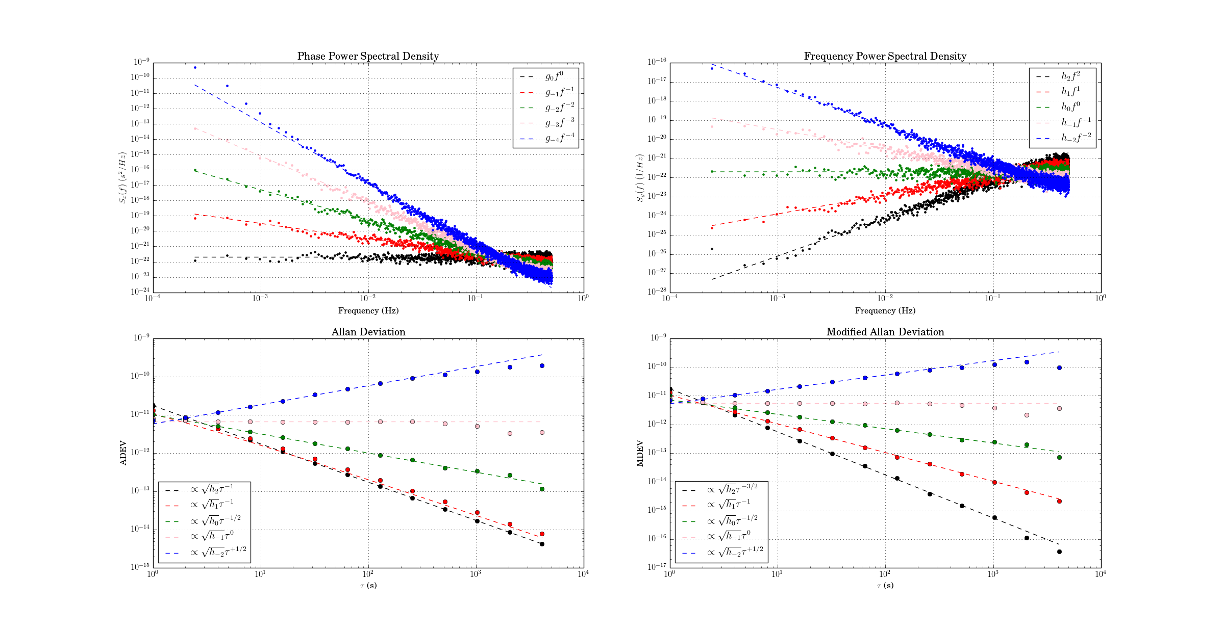
The usual noise-types studied have phase PSD noise-slopes "b" ranging from 0 to -4 (or even -5 or -6), corresponding to frequency PSD noise-slopes "a" ranging from +2 to -2 (where a=b+2). These 'colors of noise' can be visualized like this:
I've implemented three noise-identification algorithms based on Stable32-documentation and other papers: B1, R(n), and Lag-1 autocorrelation.
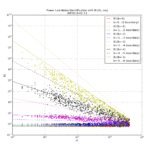
B1 (Howe 2000, Barnes1969) is defined as the ratio of the standard N-sample variance to the (2-sample) Allan variance. From the definitions one can derive an expected B1 ratio of (the length of the time-series is N)
![]()
where mu is the tau-exponent of Allan variance for the noise-slope defined by b (or a). Since mu is the same (-2) for both b=0 and b=-1 (red and green data) we can't use B1 to resolve between these noise-types. B1 looks like a good noise-identifier for b=[-2, -3, -4] where it resolves very well between the noise types at short tau, and slightly worse at longer tau.
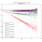
R(n) can be used to resolve between b=0 and b=-1. It is defined as the ratio MVAR/AVAR, and resolves between noise types because MVAR and AVAR have different tau-slopes mu. For b=0 we expect mu(AVAR, b=0) = -2 while mu(MVAR, b=0)=-3 so we get mu(R(n), b=0)=-1 (red data points/line). For b=-1 (green) the usual tables predict the same mu for MVAR and AVAR, but there's a weak log(tau) dependence in the prefactor (see e.g. Dawkins2007, or IEEE1139). For the other noise-types b=[-2,-3,-4] we can't use R(n) because the predicted ratio is one for all these noise types. In contrast to B1 the noise identification using R(n) works best at large tau (and not at all at tau=tau0 or AF=1).
The lag-1 autocorrelation method (Riley, Riley & Greenhall 2004) is the newest, and uses the predicted lag-1 autocorrelation for (WPM b=0, FPM b=-1, WFM b=-2) to identify noise. For other noise types we differentiate the time-series, which adds +2 to the noise slope, until we recognize the noise type.
Here are three figures for ACF, B1, and R(n) noise identification where a simulated time series with known power law noise is first generated using the Kasdin&Walter algorithm, and then we try to identify the noise slope.
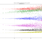
For Lag-1 ACF when we decimate the phase time-series for AF>1 there seems to be a bias to the predicted a (alpha) for b=-1, b=-3, b=-4 which I haven't seen described in the papers or understand that well. Perhaps an aliasing effect(??).
It looks like the link to Howe2000 (B1 reference) has disappeared.
The relevant paper is probably: https://doi.org/10.1109/TUFFC.2005.1509784
"Enhancements to GPS operations and clock evaluations using a "total" Hadamard deviation" in IEEE Transactions on Ultrasonics, Ferroelectrics, and Frequency Control, vol. 52, no. 8, pp. 1253-1261, Aug. 2005, doi: 10.1109/TUFFC.2005.1509784.