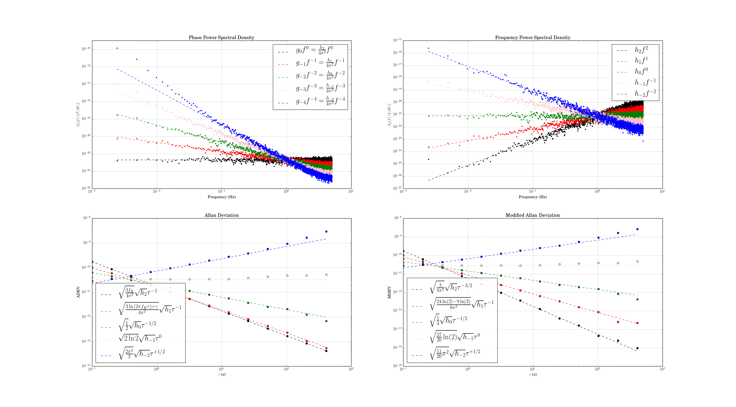
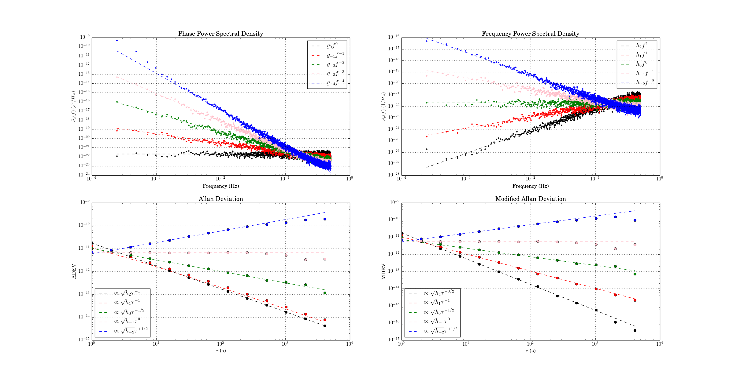
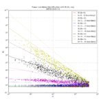
Inspired by discussion on time-nuts, here's a revised noise-colour graph. There are a few updates: The PSDs (both phase and frequency) now cross at 1 Hz (with the relation between phase-PSD and frequency-PSD explicitly stated), and the ADEV/MDEV theoretical lines now include the formula for the pre-factor (the old graph only had 'proportional to' here).
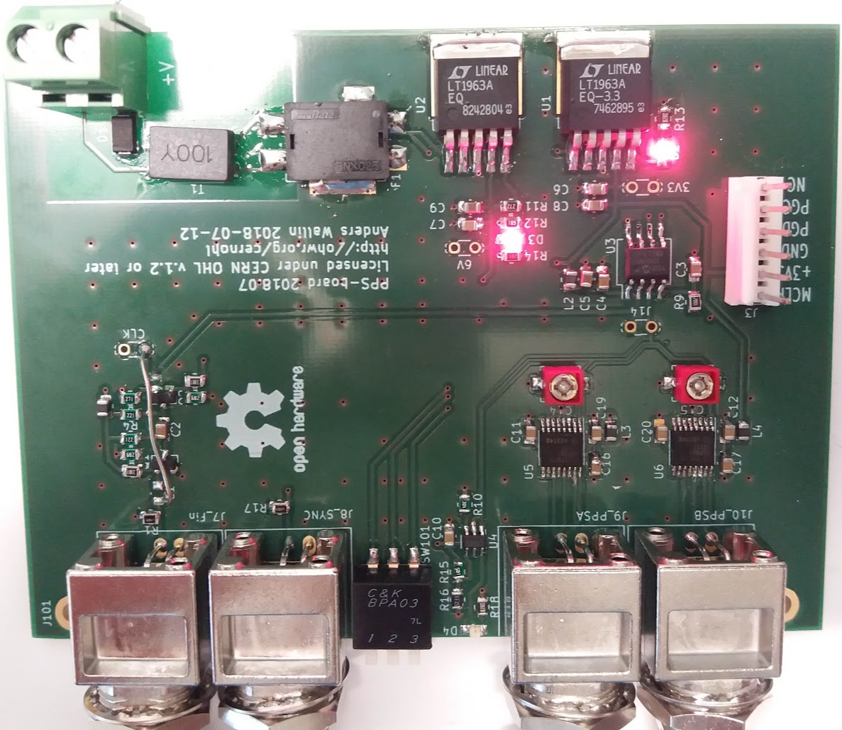
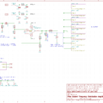
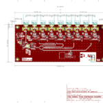
An evolution of my PICDIV-board from 2016. Takes 10MHz input and produces 1PPS (one pulse per second). This one has a TADD-2-mini inspired sine-to-square converter on the input (far left), a PIC12F675 with Tom van Baak's PICDIV-code (right), an ICSP-header for programming, and output-buffers inspired by the pulse distribution amplifier. A 3-position DIP-switch (middle left) allows config-changes, and a blinking LED indicates 1PPS (middle right).
Fixed a few bugs in the first PCB-revision and will order boards for version two soon. Eventually to be published on github/ohwr - stay tuned..
PPS-board 2018 August prototype. Note bypassed sine-to-square circuit on the left.
The usual noise-types studied have phase PSD noise-slopes "b" ranging from 0 to -4 (or even -5 or -6), corresponding to frequency PSD noise-slopes "a" ranging from +2 to -2 (where a=b+2). These 'colors of noise' can be visualized like this:
Four colors of noise. Note frequency PSD slope "a" related to phase PSD slobe "b" by a=b+2. Lower graphs show tau-slopes "mu" for ADEV and MDEV. Data point colors don't match with figures below - sorry.
I've implemented three noise-identification algorithms based on Stable32-documentation and other papers: B1, R(n), and Lag-1 autocorrelation.
B1 (Howe 2000,Barnes1969) is defined as the ratio of the standard N-sample variance to the (2-sample) Allan variance. From the definitions one can derive an expected B1 ratio of (the length of the time-series is N)
where mu is the tau-exponent of Allan variance for the noise-slope defined by b (or a). Since mu is the same (-2) for both b=0 and b=-1 (red and green data) we can't use B1 to resolve between these noise-types. B1 looks like a good noise-identifier for b=[-2, -3, -4] where it resolves very well between the noise types at short tau, and slightly worse at longer tau.
R(n) can be used to resolve between b=0 and b=-1. It is defined as the ratio MVAR/AVAR, and resolves between noise types because MVAR and AVAR have different tau-slopes mu. For b=0 we expect mu(AVAR, b=0) = -2 while mu(MVAR, b=0)=-3 so we get mu(R(n), b=0)=-1 (red data points/line). For b=-1 (green) the usual tables predict the same mu for MVAR and AVAR, but there's a weak log(tau) dependence in the prefactor (see e.g. Dawkins2007, or IEEE1139). For the other noise-types b=[-2,-3,-4] we can't use R(n) because the predicted ratio is one for all these noise types. In contrast to B1 the noise identification using R(n) works best at large tau (and not at all at tau=tau0 or AF=1).
The lag-1 autocorrelation method (Riley, Riley & Greenhall 2004) is the newest, and uses the predicted lag-1 autocorrelation for (WPM b=0, FPM b=-1, WFM b=-2) to identify noise. For other noise types we differentiate the time-series, which adds +2 to the noise slope, until we recognize the noise type.
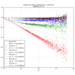
Here are three figures for ACF, B1, and R(n) noise identification where a simulated time series with known power law noise is first generated using the Kasdin&Walter algorithm, and then we try to identify the noise slope.
Lag-1 ACF noise-identification. Resolves well between all noise types at short and medium tau.
B1 noise-identification. Resolves well between b=-2…-4 at short and medium tau.
R(n) noise identification. Resolves well between b=0, -1 at medium and long tau. Note weak log(tau) dependence for b=-1 (green)
For Lag-1 ACF when we decimate the phase time-series for AF>1 there seems to be a bias to the predicted a (alpha) for b=-1, b=-3, b=-4 which I haven't seen described in the papers or understand that well. Perhaps an aliasing effect(??).
It turns out there's quirky convention of writing out the 40-character SHA1 checksum in 5 groups of 8 hex characters - whith the special undocumented rule that leading zeros are suppressed. This means the SHA1 check fails for some files where we happen to have a leading zero in one of the 8-character groups - unless you happen to know about the undocumented rule...
The output looks like this. "New" is the checksum computed by the program, "Old" is the checksum contained in the published file.
There's also another simple script for authoring a leap-seconds.list file. It might be used for adding an artificial leap-second, generating a leap-seocnds.list file, and testing how different devices react to a leap-second - without having to wait for a real leap-second event.
Following the publication of Circular-T nr. 357 we shall take a look at the RMS error of UTC-UTC(k) in different laboratories across the world. Should we rank the 75 laboratories that have complete UTC-UTC(k) records by RMS error for this month we find the following.
Warning: Past performance is not an indicator of future results.
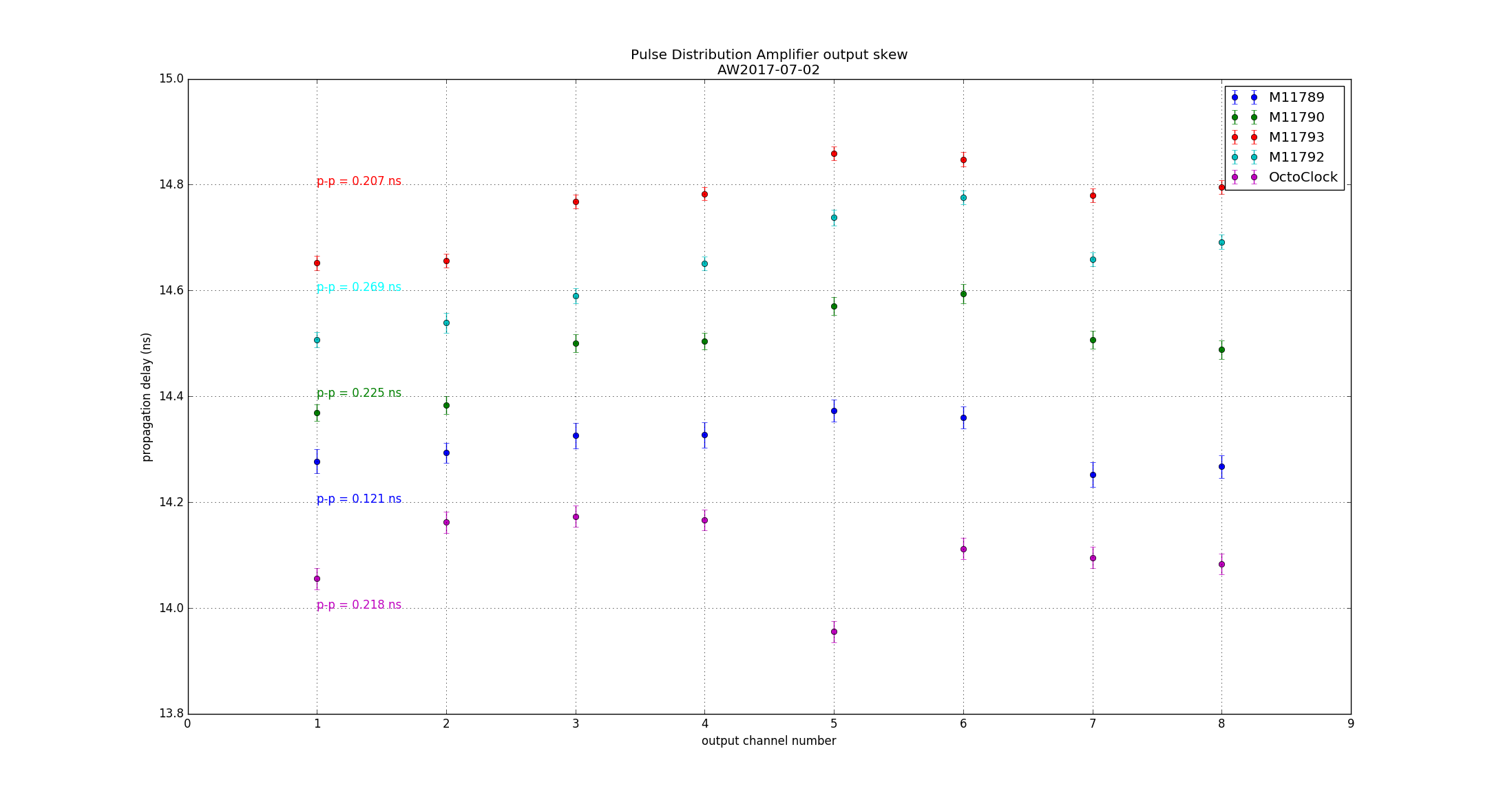
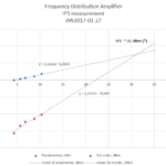
Here is the measured output delay skew from four of my "PDA 2017.01" designs, based on LT1711 comparator driving a 74AC14 schmidt trigger which in turn drives eight 74AC04 output-stages.
Although the PCB was designed with equal-length traces for the output stages it appears that channels 3-4 and 5-6 are consistently late, and some shortening of the traces would improve things. I tried this on one PCB (blue data points) with moderate success.
Measurement setup: 1PPS source to 50-ohm splitter. One output of the splitter drives CH1(start) of a time interval counter (HPAK 53230A), the other output drives the input of the pulse distribution amplifier. Outputs wired to CH2(stop) of the counter and measured for 100 s or more (delay is average of 100 pulses). Counter inputs DC-coupled, 50 Ohms, trigger level 1.0 V.
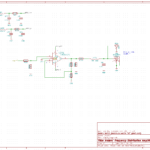
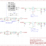
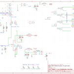
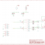
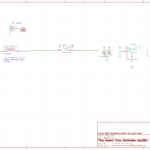
1:8 frequency distribution amplifier based on LMH6702 and LMH6609 op-amps.
In particular the power-supply section using a common-mode choke, a Murata BNX025 filter, and low-noise regulators LT1963 and LT3015 seems to work quite well. I also used ferrites (2 kOhm @ 100 MHz) as well as an RC-filter on all supply pins. Perhaps overkill? Performance with the intended AC/DC brick is still to be verified.
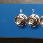
Board design with either SMA or BNC connectors spaced 16mm apart.
Input stage
Output stage
Supply filtering and regulation
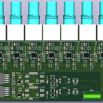
PCB in KiCad. Voltage regulators get quite hot so should move away from the op-amps in the next revision.
3D models (partly) in KiCad.
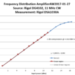
Measurements around 10 MHz show a 1 dB compression at over 14 dBm and an IP3 of around 27 to 30 dBm. The gain extends beyond 100 MHz with some gain-peaking.
IP3 measurement using two tones around 10MHz and looking at the IMD components
Gain and compression measurement at 10 MHz.
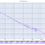
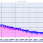
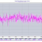
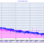
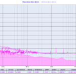
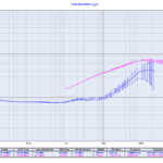
Some measurements of residual phase-noise with a 3120A phase-meter, at 10 MHz. My earlier distribution amplifier required shielding with aluminium foil as well as powering from a lead-acid battery to achieve a reasonably quiet phase-noise spectrum. These measurements were done with lab power-supplies for +/-12 V to the board and without any shielding.
ADEV
AM noise. Note that noise-floor measurement run is shorter than actual amplifier measurement.
Phase-residual over 12 hours.
Phase-noise.
PN and AM.
TDEV
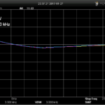
Finally some measurements of gain vs. frequency with a Rigol spectrum analyzer.
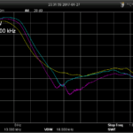
Gain flatness around 10 MHz for output channels 1, 4, and 8.
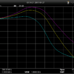
Gain-peaking for original design. Channels 1, 4, and 8 left to right.
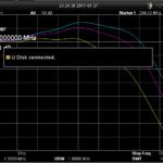
More moderate gain-peaking after adding 100pF cap to output stage. Again from left to right channels 1, 4, and 8.
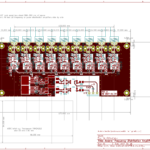
A new pulse distribution amplifier for 1PPS distribution.
The input is fed to a LT1711 comparator triggering at 1.0 V (set by reference ADR423). This edge is buffered by 74AC14 before 1:8 fan-out to output-stages with three 74AC04 inverters in parallel driving the outputs.
Preliminary measurements show around 200ps channel-to-channel propagation skew - to be improved on by further trace-length matching or tuning. More measurements to follow.
Input section. LT1711 comparator triggers at level set by voltage reference. 74AC14 buffer to 1:8 fan-out for output stages.
Output sections. Three 74AC04 inverters in parallel.
Supply section. LT1963A fed via common-mode choke and BNX025 filter.
Board design. To fit either BNC or SMA connectors, spaced 16mm apart.
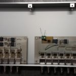
A new distribution amplifier design featuring a 1PPS pulse distribution amplifier (PDA) and a 5/10 MHz frequency distribution amplifier (FDA).
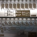
1U 150mm deep rack-enclosure from Schaeffer. Prototype PCBs without soldermask or silkscreen from Prinel. Both the FDA and PDA boards have 1:8 fan-out with 9 BNC (optionally SMA) connectors spaced 16mm apart. The boards fit comfortably side-by side on a 19" rack panel. Some funky BNC-cables with unusually large connectors may not fit side-by-side 16mm apart - a price to pay for the compact design. The plan is to use an +/-12 AC/DC brick power-supply (not shown) which fits in the back of the enclosure.
Detailed posts on the PDA and FDA boards to follow.
1U front-panel.
FDA (left) and PDA(right) in enclosure. AC power entry top left. Space for AC/DC power-supply at the top.
Bare prototype boards for PDA and FDA. No soldermask or silkscreen.
