Fun with Chi-Squared

As mentioned before, the Chi-Squared inverse cumulative distribution is used when calculating confidence intervals in allantools.

When comparing computed confidence intervals against Stable32, there seems to be some systematic offsets, which I wanted to investigate.

While allantools uses scipy.stats.chi2.ppf(), It turns out that Stable32 uses an iterative method for EDF<=100, and an approximation from Abramowitz and Stegun: Handbook of Mathematical Functions for EDF>100. This 1964 book seems to be available online from many sites. The approximation (for large EDF) for the inverse chi-squared cumulative distribution is equations 26.4.17 (p410 in the PDF) (here nu is the equivalent degrees of freedom)

Abramowitz and Stegun, inverse chi-squared cumulative distribution, for large EDF.

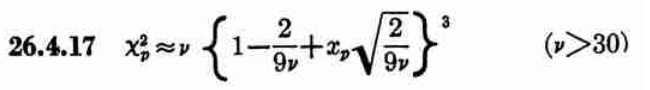
Where xp is from the inverse of the Normal cumulative distribution, computed via the approximation 26.2.22 (p404 in the PDF)

Abramowitz & Stegun, approximate inverse Normal cumulative distribution, for 0<p<0.5

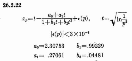
It also looks like the Stable32 source contains a misprint, where the a1 coefficient of 26.2.22 is used with two digits in the wrong order! (I did promise 'fun' in the title of this post!)

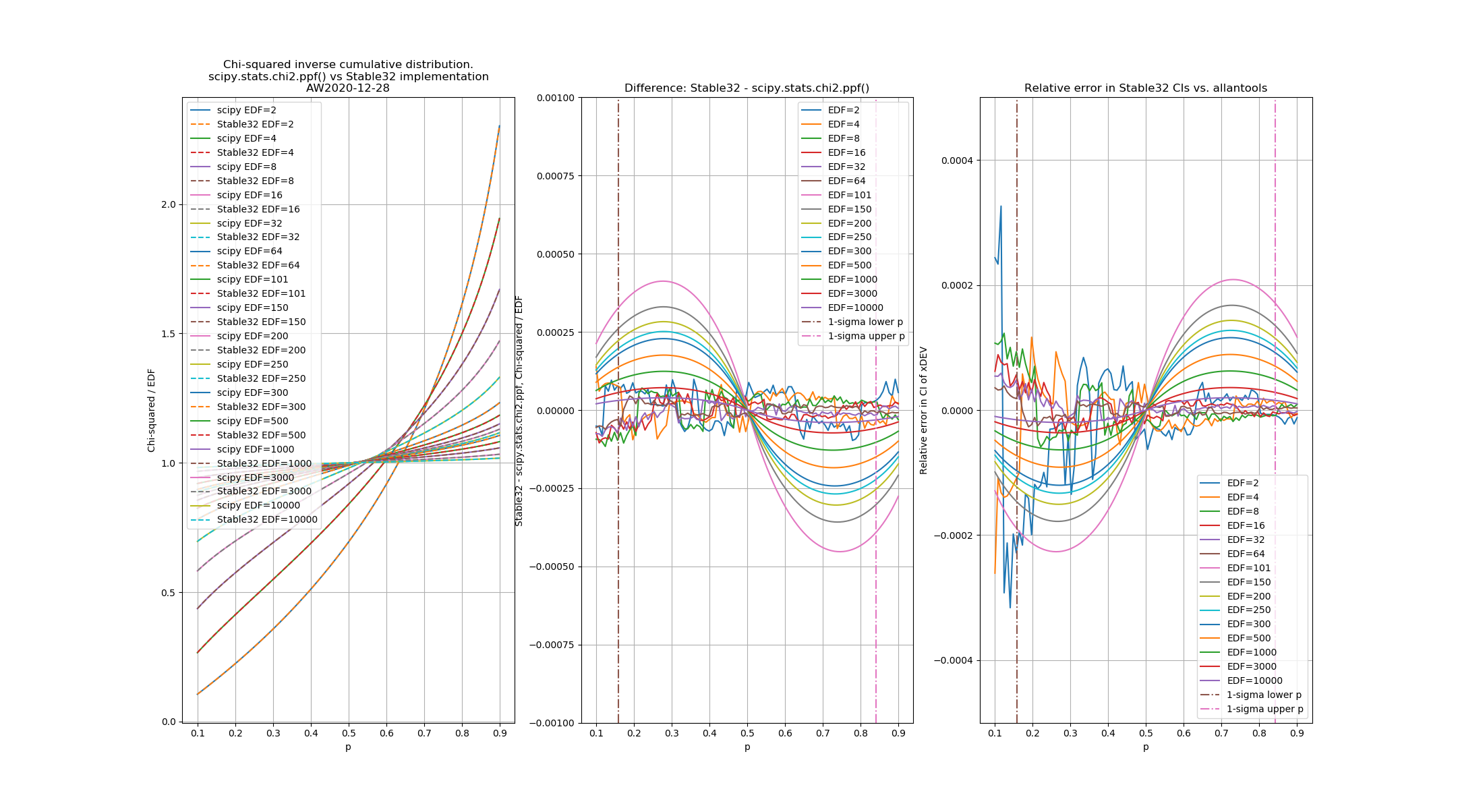
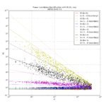
a1=0.27601   # typo in the Stable32 source code!? should be 0.27061

If we plot both scipy.stats.chi2.ppf() and the Stable32 implementation for various EDF and probabilities we get the following:

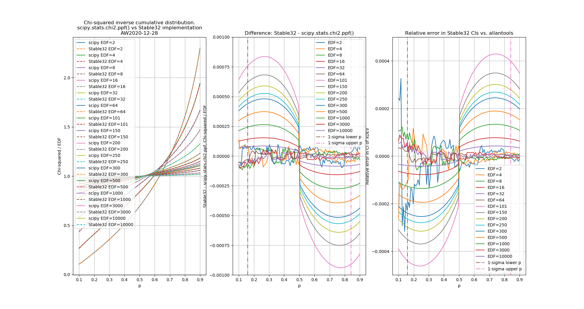
The leftmost figure shows Chi-Squared values (divided by EDF, to overlap all curves). There's not much difference between scipy and Stable32 visible at this scale. The middle figure shows the difference between the two algorithms. This shows very clearly the small (<100) EDF-region where the iterative algorithm in Stable32 produces a Chi-squared value in agreement with scipy to better than 4 digits (see the noisy traces around zero). This plot also reveals the shortcomings of the Abramovitz & Stegun approximation, together with the source-code misprint. The errors are largest, up to almost 1e-3 (in chi-squared/EDF) for EDF=101, and decrease with higher EDF. The rightmost figure shows what impact this has on computed confidence intervals - shown as relative errors. The confidence interval is proportional to sqrt(EDF/chi-squared). The dashed lines show the probabilities corresponding to 1-sigma confidence intervals, where we usually sample this function.

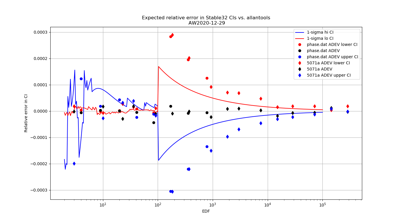
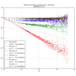
For 1-sigma confidence intervals we can now compare computed results with Stable32 and allantools to the comparison above of scipy and Abramovitz&Stegun + misprint.

Predicted and computed relative error for confidence intervals computed with Stable32 vs. allantools. The lower bound is shown in red, and the upper bound in blue. The relative error of the computed ADEV is shown as black symbols, for reference. The symbols are from computed deviations and confidence intervals for two test-datasets in allantools: phase.dat and a 5071a-dataset.

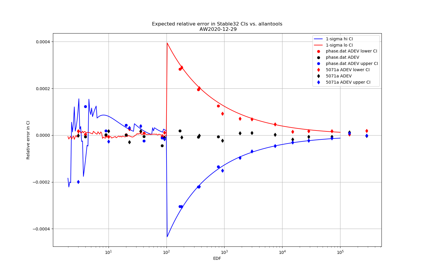
Are we having fun yet!? The comparison above between the two methods to compute the inverse chi-squared cumulative distribution seems to predict how Stable32 confidence intervals differ from allantools confidence intervals quite well! Note that Stable32 results are copy/pasted from the GUI with 5 significant digits, so some noise at the 1e-4 level is to be expected. Note that the relative error has a different sign depending on if we look at the lower or upper bound, and also depending on if we use the EDF<=100 iterative algorithm or the EDF>100 Abramovitz&Stegun+misprint approximation. For large EDF the upper bound (blue) of Stable32 is a bit too low, while the lower bound (red) is a bit too high.

Finally, the chi-squared figure and the expected confidence interval relative error figure, if we fix the misprint in the a1 coefficient:

Note with the a1-coefficient misprint fixed the approximation is exact at p=0.5, and there is no discontinuity in the difference-curves.

If the a1-coefficient misprint would be fixed in Stable32, we could expect the EDF>100 confidence interval relative errors between Stable32 and allantools to be roughly halved. The data-symbols are the same as in the figure above - agreement between the lines and symbols is not expected here.

Python code for producing these figures is available: chi2_stable32.py

The approximations used by Stable32 are not (yet?) included in allantools.

Faster mtotdev() and htotdev()

The AllanTools functions mtotdev() and htotdev() are now almost 10-times faster, after an update to the code that more efficiently calculates moving averages.

The old code used numpy.mean() for each iteration of a loop:

for j in range(0, 6*m): # summation of the 6m terms.
    xmean1 = np.mean(xstar[j     :   j+m])
    xmean2 = np.mean(xstar[j+m   : j+2*m])
    xmean3 = np.mean(xstar[j+2*m : j+3*m])

However this can be computed much faster by noticing that the new mean differs from the old (already computed!) mean by just two points, one at the start is dropped, and a new one at the end is added:

for j in range(0, 6*m): # summation of the 6m terms.
    if j == 0:
        # intialize the sum
        xmean1 = np.sum( xstar[0:m] )
        xmean2 = np.sum( xstar[m:2*m] )
        xmean3 = np.sum( xstar[2*m:3*m] )
    else:
        # j>=1, subtract old point, add new point
        xmean1 = xmean1 - xstar[j-1] + xstar[j+m-1] #
        xmean2 = xmean2 - xstar[m+j-1] + xstar[j+2*m-1] #
        xmean3 = xmean3 - xstar[2*m+j-1] + xstar[j+3*m-1] #

Noise Colours - again

Inspired by discussion on time-nuts, here's a revised noise-colour graph. There are a few updates: The PSDs (both phase and frequency) now cross at 1 Hz (with the relation between phase-PSD and frequency-PSD explicitly stated), and the ADEV/MDEV theoretical lines now include the formula for the pre-factor (the old graph only had 'proportional to' here).

Source: example_noise_slopes2.py

Simulated time-series with power-law noise. The relation between phase-PSD, frequency-PSD, ADEV, and MDEV is shown.

It is left as an exercise to the reader to properly explain the ADEV pre-factor for flicker-phase noise :).

Power Law Noise Identification for AllanTools

For AllanTools statistics both bias-correction and confidence interval calculation requires identifying the dominant power law noise in the input time-series.

The usual noise-types studied have phase PSD noise-slopes "b" ranging from 0 to -4 (or even -5 or -6), corresponding to frequency PSD noise-slopes "a" ranging from +2 to -2 (where a=b+2). These 'colors of noise' can be visualized like this:


Four colors of noise. Note frequency PSD slope "a" related to phase PSD slobe "b" by a=b+2. Lower graphs show tau-slopes "mu" for ADEV and MDEV. Data point colors don't match with figures below - sorry.

I've implemented three noise-identification algorithms based on Stable32-documentation and other papers: B1, R(n), and Lag-1 autocorrelation.

B1 (Howe 2000, Barnes1969) is defined as the ratio of the standard N-sample variance to the (2-sample) Allan variance. From the definitions one can derive an expected B1 ratio of (the length of the time-series is N)

where mu is the tau-exponent of Allan variance for the noise-slope  defined by b (or a). Since mu is the same (-2) for both b=0 and b=-1  (red and green data) we can't use B1 to resolve between these noise-types. B1 looks like a good noise-identifier for b=[-2, -3, -4] where it resolves very well between the noise types at short tau, and slightly worse at longer tau.

R(n) can be used to resolve between b=0 and b=-1. It is defined as the ratio MVAR/AVAR, and resolves between noise types because MVAR and AVAR have different tau-slopes mu. For b=0 we expect mu(AVAR, b=0) = -2 while mu(MVAR, b=0)=-3 so we get mu(R(n), b=0)=-1 (red data points/line). For b=-1 (green) the usual tables predict the same mu for MVAR and AVAR, but there's a weak log(tau) dependence in the prefactor (see e.g. Dawkins2007, or IEEE1139). For the other noise-types b=[-2,-3,-4] we can't use R(n) because the predicted ratio is one for all these noise types. In contrast to B1 the noise identification using R(n) works best at large tau (and not at all at tau=tau0 or AF=1).

The lag-1 autocorrelation method (Riley, Riley & Greenhall 2004) is the newest, and uses the predicted lag-1 autocorrelation for (WPM b=0, FPM b=-1, WFM b=-2) to identify noise. For other noise types we differentiate the time-series, which adds +2 to the noise slope, until we recognize the noise type.

Here are three figures for ACF, B1, and R(n) noise identification where a simulated time series with known power law noise is first generated using the Kasdin&Walter algorithm, and then we try to identify the noise slope.

For Lag-1 ACF when we decimate the phase time-series for AF>1 there seems to be a bias to the predicted a (alpha) for b=-1, b=-3, b=-4 which I haven't seen described in the papers or understand that well. Perhaps an aliasing effect(??).


AllanTools 2016.11 - now with Confidence Intervals!

at2016-11_wtih_ci

I've added confidence interval estimation to allantools, based on a 2004 paper by Greenhall & Riley: "Uncertainty of stability variances based on finite differences"

So far not much is automated so you have to run everything manually. After a normal call to allantools.adev() to calculate the ADEV we loop through each (tau, adev) pair and first call allantools.edf_greenhall() to get the number of equivalent-degrees-of-freedom (EDF), and then evaluate a confidence interval with allantools.confidence_interval(). A knowledge or estimate of the noise type "alpha" is required for edf_greenhall() - here we just assume alpha=0.

This example is on github at: https://github.com/aewallin/allantools/blob/master/examples/ci_demo.py

import numpy
import matplotlib.pyplot as plt
 
import allantools as at
 
# this demonstrates how to calculate confidence intervals for ADEV
# using the algorithms from Greenhall2004
data_file = '../tests/phasedat/PHASE.DAT'
 
def read_datafile(filename):
    p = []
    with open(filename) as f:
        for line in f:
            if not line.startswith("#"):  # skip comments
                p.append(float(line))
    return p
 
# read input data from file
phase = read_datafile(data_file)
# normal ADEV computation, giving naive 1/sqrt(N) errors
(taus,devs,errs,ns) = at.adev(phase, taus='octave')
 
# Confidence-intervals for each (tau,adev) pair separately.
cis=[]
for (t,dev) in zip(taus,devs):
    # Greenhalls EDF (Equivalent Degrees of Freedom)
    # alpha     +2,...,-4   noise type, either estimated or known
    # d         1 first-difference variance, 2 allan variance, 3 hadamard variance
    #           we require: alpha+2*d >1     (is this ever false?)
    # m         tau/tau0 averaging factor
    # N         number of phase observations
    edf = at.edf_greenhall( alpha=0, d=2, m=t, N=len(phase), overlapping = False, modified=False )
    # with the known EDF we get CIs 
    # for 1-sigma confidence we set
    # ci = scipy.special.erf(1/math.sqrt(2)) = 0.68268949213708585
    (lo,hi) = at.confidence_intervals( dev=dev, ci=0.68268949213708585, edf=edf )
    cis.append( (lo,hi) )
 
# now we are ready to print and plot the results
print "Tau\tmin Dev\t\tDev\t\tMax Dev"
for (tau,dev,ci) in zip(taus,devs,cis):
    print "%d\t%f\t%f\t%f" % (tau, ci[0], dev, ci[1] )
""" output is
Tau	min Dev		Dev		Max Dev
1	0.285114	0.292232	0.299910
2	0.197831	0.205102	0.213237
4	0.141970	0.149427	0.158198
8	0.102541	0.110135	0.119711
16	0.056510	0.062381	0.070569
32	0.049153	0.056233	0.067632
64	0.027109	0.032550	0.043536
128	0.026481	0.033855	0.055737
256	0.007838	0.010799	0.031075
"""
plt.figure(figsize=(12,8))
plt.gca().set_yscale('log')
plt.gca().set_xscale('log')
err_lo = [ d-ci[0] for (d,ci) in zip(devs,cis)]
err_hi = [ ci[1]-d for (d,ci) in zip(devs,cis)]
 
plt.errorbar(taus, devs, yerr=[ err_lo, err_hi ] ,fmt='o')
plt.grid()
plt.xlabel('Tau (s)')
plt.ylabel('ADEV')
plt.title('AllanTools 2016.11 - now with Confidence Intervals!')
# just to check plot the intervals as dots also
plt.plot(taus, [ci[0] for ci in cis],'r.')
plt.plot(taus, [ci[1] for ci in cis],'g.')
 
plt.show()

scipy.stats.chi2.ppf() without scipy

Allantools has a dependence on scipy because it uses scipy.stats.chi2.ppf() (inverse of the chi-squared cumulative distribution function) in the code for confidence intervals.

When testing scipy takes quite a long time to install and the whole package seems a bit overkill for just this one function.

So I tried implementing it using just numpy. It sort of works, but not for corner cases where p is very close to 1.0 or k is a big number. I get for example:

    top = pow(x, s)*math.exp(-x)*pow(x,k)
OverflowError: (34, 'Numerical result out of range')

Maybe there's something trick when numerically evaluating lower_gamma() using the series expansion that I am missing...

import scipy.stats
import math
import numpy
 
def bisection(function, k, p, a, b, tol):
	# http://code.activestate.com/recipes/578417-bisection-method-in-python/
	assert (function(a,k)-p)*(function(b,k)-p) < 0 # a, b must bracket root
	c = (a+b)/2.0
	while (b-a)/2.0 > tol:
		if (function(c, k)-p) == 0:
			return c
		elif (function(a,k)-p)*(function(c,k)-p) < 0:
			b = c
		else :
			a = c
		c = (a+b)/2.0
	return c
 
def lower_gamma(s,x):
	# lower incomplete gamma function
	# https://en.wikipedia.org/wiki/Incomplete_gamma_function#Evaluation_formulae
	g  = 0
	last_g = 1.0
	done = False
	tol = 1.0e-6
	k=0
	while not done:
		top = pow(x, s)*math.exp(-x)*pow(x,k)
		bot = numpy.prod( [float(s+j) for j in range(k+1) ] )
		dg = float(top)/float(bot)
		if dg == float("Inf"):
			break
		g += dg
		k += 1
		if k>100: # get at least 100 terms in the sum
			if g==0:
				break
			delta = abs(dg/g)
			if delta == float("Inf"):
				break
			if delta < tol:
				done = True
		last_g = g
	return g
 
def chi2_cdf(x, k):
	# chi-squared cumulative density function
	# cdf(x; k) = lower_gamma(k/2, x/2) / gamma(k/2)
	return lower_gamma(k/2.0, x/2.0) / math.gamma(k/2.0)
 
def chi2_ppf(p, k):
	# chi-squared Percent point function (inverse of cdf percentiles).
	# look for x such that
	# p = chi2_cdf( x=chi2_ppf(p, k), k)
	tol = 1e-8
	lolim = 0
	hilim = k
	while (chi2_cdf(lolim,k)-p)*(chi2_cdf(hilim,k)-p) > 0: 
		hilim *= 1.5
	return bisection( chi2_cdf, k, p, lolim, hilim, tol)
 
print "scipy cdf: ",scipy.stats.chi2.cdf(55, 33)	
print "own   cdf: ",chi2_cdf(55, 33)
 
 
print "scipy ppf ", scipy.stats.chi2.ppf(0.4, 33)
print "  own ppf ", chi2_ppf(0.4, 33)
 
# test that we really found the inverse
print scipy.stats.chi2.cdf(scipy.stats.chi2.ppf(0.4, 33), 33)
print chi2_cdf( chi2_ppf(0.4, 33), 33 )
 
# try to check the scipy function against our own function
# for some random input of (p, k)
for n in range(100):
	k = numpy.random.randint(20, 200)
	p = numpy.random.random()
	print k, p,
	a=scipy.stats.chi2.ppf(p, k)
	b=chi2_ppf(p, k)
	ok = numpy.isclose(a, b)
	if ok:
		print  ok
	else:
		print  ok, a, b
	assert ok