Opencamlib cutter shapes

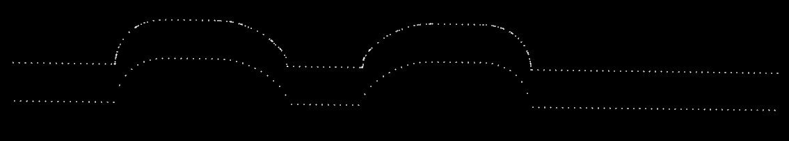
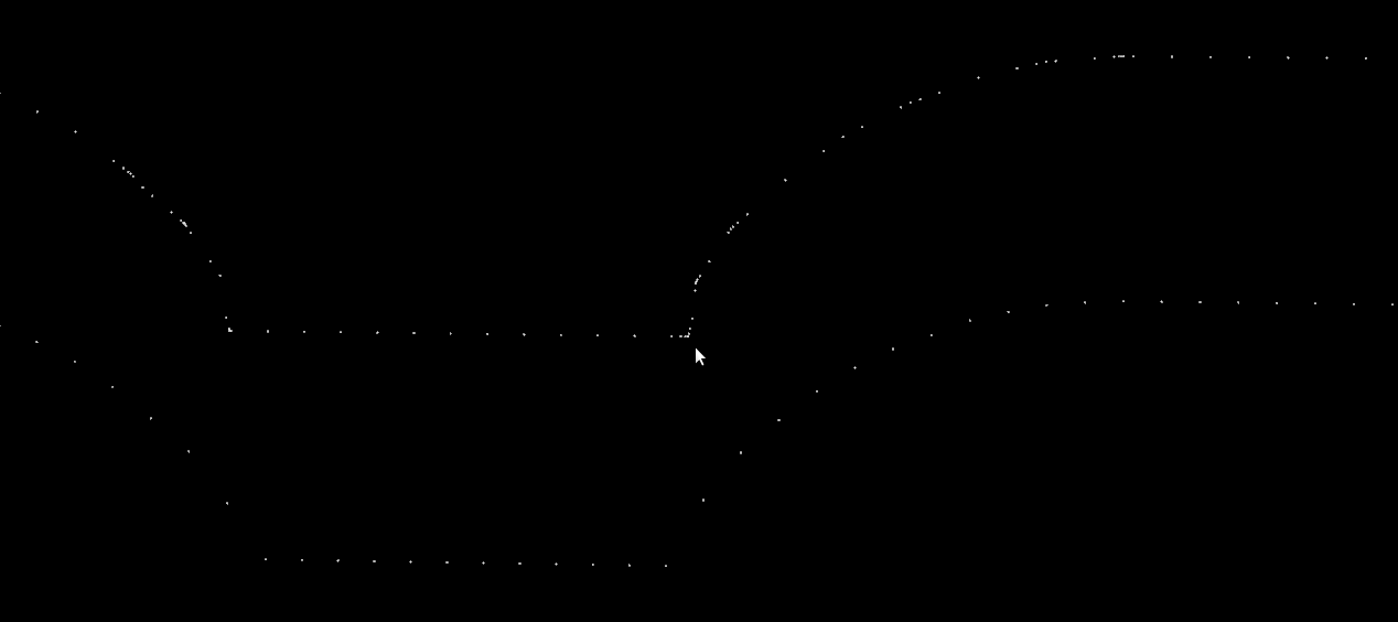
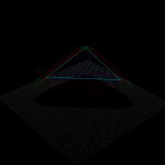
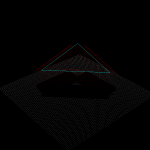
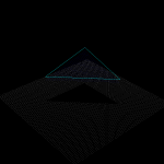
If you calculate toolpaths around a very narrow and 'pointy' triangle you will get toolpaths in the shape of the inverse cutter - the "Inverse Tool Offset". Here I've plotted the basic operations, in red/blue drop-cutter which drops the cutter down along the z-axis until it contacts the triangle, and in cyan waterlines which are the results of a push-cutter operation that pushes the cutter at constant z-height along the x/y axis into contact with the triangle.

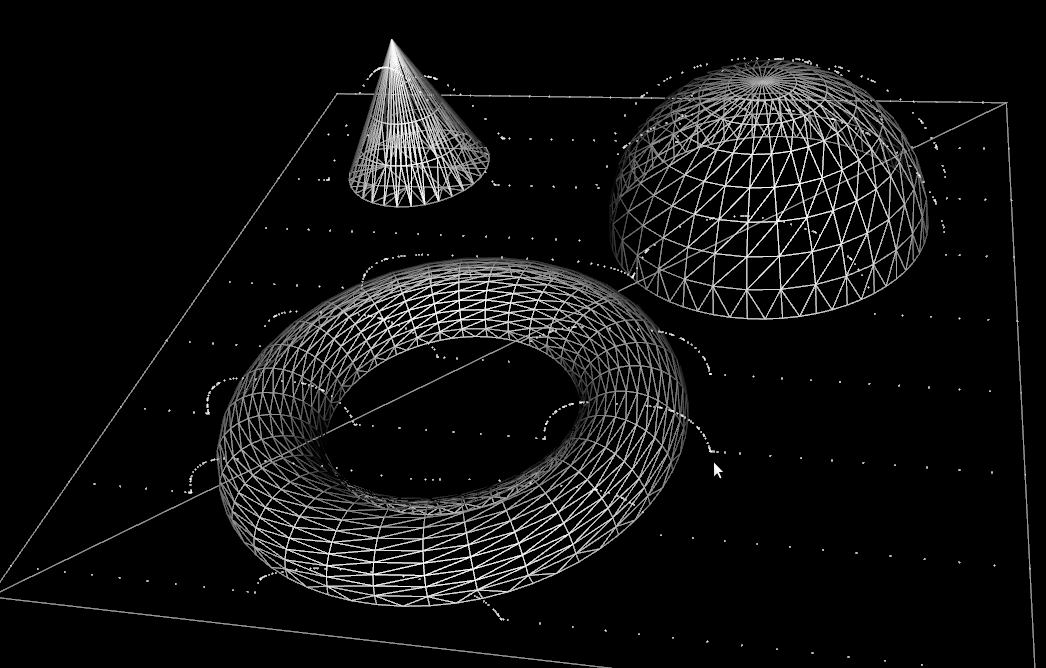
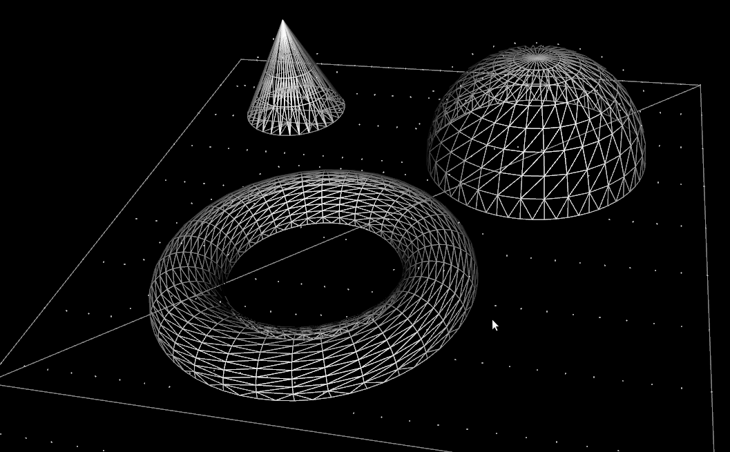
There are four basic cutter shapes: (1) Cylinder, (2) Sphere('Ball'), (3) Toroid('Bull'), and (4) Cone. The triangle contact can be divided into tests for contact with (a) the three vertices of the triangle, (b) the facet of the triangle, and (c) the three edges of the triangle. That's 4x3 = 12 contact/collision-test functions that have to be written (a few, particularly the facet-tests, can be combined into one base-class method).

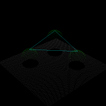
Once the basic cutter shapes work it is possible to combine them through CompositeCutter. The bottom row shows cutters with a central part corresponding to the top row of cutters, and a conical outer part.

The point of this exercise is of course not only to plot inverse-tool-shapes, but to be able to calculate toolpaths for these and other CompositeCutter tool shapes. This will become more interesting if/when the cutting-simulation starts working and it will be possible to compare for example surface-finish vs. cutting-time of a BallCutter operation vs. a BullCutter operation.

Adaptive sampling drop-cutter

Inspired by this post on the pycam forum and by this 1993 paper by Luiz Henrique de Figueiredo (or try another version) I did some work with adaptive sampling and drop-cutter today.

The point based CAM approach in drop-cutter, or axial tool-projection, or z-projection machining (whatever you want to call it) is really quite similar to sampling an unknown function. You specify some (x,y) position which you input to the drop-cutter-oracle, which will come back to you with the correct z-coordinate. The tool placed at this (x,y,z) will touch but not gouge the model. Now if we do this at a uniform (x,y) sampling rate we of course face the the usual sampling issues. It's absolutely necessary to sample the signal at a high enough sample-rate not to miss any small details. After that, you can go back and look at all pairs of consecutive points, say (start_cl, stop_cl). You then compute a mid_cl which in the xy-plane lies at the mid-point between start_cl and stop_cl and, call drop-cutter on this new point, and use some "flatness"/collinearity criterion for deciding if mid_cl should be included in the toolpath or not (deFigueiredo lists a few). Now recursively run the same test for (start_cl, mid_cl) and (mid_cl, stop_cl). If there are features in the signal (like 90-degree bends) which will never make the flatness predicate true you have to stop the subdivision/recursion at some maximum sample rate.

Here the lower point-sequence (toolpath) is uniformly sampled every 0.08 units (this might also be called the step-forward, as opposed to the step-over, in machining lingo). The upper curve (offset for clarity) is the new adaptively sampled toolpath. It has the same minimum step-forward of 0.08 (as seen in the flat areas), but new points are inserted whenever the normalized dot-product between mid_cl-start_cl and stop_cl-mid_cl is below some threshold. That should be roughly the same as saying that the toolpath is subdivided whenever there is enough of a bend in it.

The lower figure shows a zoomed view which shows how the algorithm inserts points densely into sharp corners, until the minimum step-forward (here quite arbitrarily set to 0.0008) is reached.

If the minimum step-forward is set low enough (say 1e-5), and the post-processor rounds off to three decimals of precision when producing g-code, then this adaptive sampling could give the illusion of "perfect" or "correct" drop-cutter toolpaths even at vertical walls.

The script for drawing these pics is: http://code.google.com/p/opencamlib/source/browse/trunk/scripts/pathdropcutter_test_2.py

Here is a bigger example where, to exaggerate the issue, the initial sample-rate is very low:

Drop-Cutter examples

I've experimented with using OpenMP to calculate drop-cutter toolpaths on a quad-core machine. These now run reasonably fast. There are obvious lurking bugs with BallCutter and BullCutter still...

Code is here: code.google.com/p/opencamlib/ (if you know C++, computational geometry, and cnc-machining, or are willing to learn, this project needs your help!)

See also: styrofoam spider

Toroidal drop-cutter

A one-triangle test of drop-cutter for toroidal tools (a.k.a. filleted-endmills, or bull-nose).

The blue points are contacts with the facet, and the green points are contacts with the vertices. These are easy.

The edges-contacts (red-points) are a bit more involved, and are done with the offset-ellipse solver presented earlier here(the initial geometry) and here(offset-ellipse construction) and here(convergence of the solver) and here(toroid-line intesection animation).

Offset ellipse, part 2

More on the offset-ellipse calculation, which is related to contacting toroidal cutters against edges(lines). An ellipse aligned with the x- and y-axes, with axes a and b can be given in parametric form as (a*cos(theta) , b*sin(theta) ). The ellipse is shown as the dotted oval, in four different colours.

Now the sin() and cos() are a bit expensive the calculate every time you are running this algorithm, so we replace them with parameters (s,t) which are both in [-1,1] and constrain them so s^2 + t^2 = 1, i.e. s = cos(theta) and t=sin(theta). Points on the ellipse are calculated as (a*s, b*t).

Now we need a way of moving around our ellipse to find the one point we are seeking. At point (s,t) on the ellipse, for example the point with the red sphere in the picture, the tangent(shown as a cyan line) to the ellipse will be given by (-a*t, b*s). Instead of worrying about different quadrants in the (s,t) plane, and how the signs of s and t vary, I thought it would be simplest always to take a step in the direction of the tangent. That seems to work quite well, we update s (or t) with a new value according to the tangent, and then t (or s) is calculated from s^2+t^2=1, keeping the sign of t (or s) the same as it was before.

Now for the Newton-Rhapson search we also need a measure of the error, which in this case is the difference in the y-coordinate of the offset-ellipse point (shown as the green small sphere, and obviously calculated as the ellipse-point plus the offset-radius times a normal vector) and where we want that point. Then we just run the algorithm, always stepping either in the positive or negative direction of the tangent along the ellipse, until we reach the required precision (or max number of iterations).

Here's an animation which first shows moving around the ellipse, and then at the end a slowed-down Newton-Rhapson search which in reality converges to better than 8 decimal-places in just seven (7) iterations, but as the animation is slowed down it takes about 60-frames in the movie.

I wonder if all this should be done in Python for the general case too, where the axes of the ellipse are not parallel to the x- and y-axes, before embarking on the c++ version?

Offset ellipse

Contacting a toroidal cutter (not shown) against an edge (cyan line), is equivalent to dropping down a cylindrical cutter (lower edge shown as yellow circle) against a cylinder (yellow tube) around the edge, with a radius equal to the tube-radius of the original toroidal cutter.

The plane of the tip of the cylindrical cutter slices through the yellow tube and produces an ellipse (inner green and red points). The way this example was rotated it is  obvious where the center of the ellipse along the Y-coordinate (along the green arrow) should lie. But the X-coordinate (along the red arrow) is unknown. One way of finding out is to realise that the center of the original toroidal cutter (white point) must lie on an offset-ellipse (outer green/red points). Once the X and Y coordinates are known it is fairly straightforward to find out the cutter-contact point between the cylindrical cutter and the tube, and from that the cutter-contact point between the toroid and the edge. Finally from that the cutter-location can be found.

Something to implement in opencamlib soon...

Spherical drop-cutter

For spherical cutters (a.k.a. ball-nose), the vertex-test (green dots), and the facet-test (blue dots), are fairly trivial. The edge-test (red-dots) is slightly more involved. Here, unlike before, I tried doing it without too many calls to "expensive" functions like sin(), cos() and sqrt(). The final result of taking the maximum of all tests is shown in the "all" image which shows cutter-locations colour-coded based on the type of cutter-contact.

The logical next step is the toroidal, or bull-nose cutter. Again the edge-test is the most difficult, and I never really understood where the geometry of the offset-ellipse shows up... anyone care to explain?

Drop-cutter Tux

After the kd-tree search is done, I've added an overlap-check which leaves only triangles with a bounding box intersecting the cutter's bounding box for the drop-cutter algorithm. It's seems like a band-aid kind of hack to get it working, I think if the tree-search would be bug free the overlap check would not be needed...

The HD-version of the video is much better, once youtube has finished processing.

Youtube vs. Vimeo

I've continued to translate into C++ the old cam-experiments I wrote in C#. The kd-tree search for which triangles lie under the cutter seems to work, and the best way to visualize what is going on is through a video. Trying Vimeo for a change, to see if it's any better than youtube for these CAD/CAM-visualizations, since they advertise HD.

There are 360 original frames captured from VTK, and the original was created with

mogrify -format jpg -quality 97 *.png

followed by (copy/pasted from some site google found for me...)

mencoder mf://*.jpg -mf fps=25:type=jpg  -aspect 16:9 -of lavf -ovc lavc -lavcopts aglobal=1:vglobal=1:coder=0:vcodec=mpeg4:vbitrate=4500 -vf scale=1280:720 -ofps 30000/1001 -o OUTPUT3.mp4

If anyone knows something better which produces nice results on youtube or vimeo, let me know.

The original is 1280x720 pixels, so it's better to jump out of the blog to watch the videos in native resolution.

Youtube: http://www.youtube.com/watch?v=k3uCpWYm174

Vimeo: http://vimeo.com/10215501

Drop-cutter toolpath algorithm development, part1 from anders wallin on Vimeo.

OK, so the video doesn't really show what is going on with the kd-tree search at all 🙂 . It only shows two toolpaths, one coloured in many colours which is calculated without the kd-tree, and another one (offset upwards for clarity) that is calculated, much faster, using the kd-tree.