With new thicker solid mu-metal magnetic shields (2 layers), the clock transition in our 88Sr+ experiments shows a transform-limited linewidth of ca 10 Hz using a 72ms probe pulse. More testing to follow, as we try to lengthen the probe-pulse and search for the ultimate linewidth limit.
Category: Research
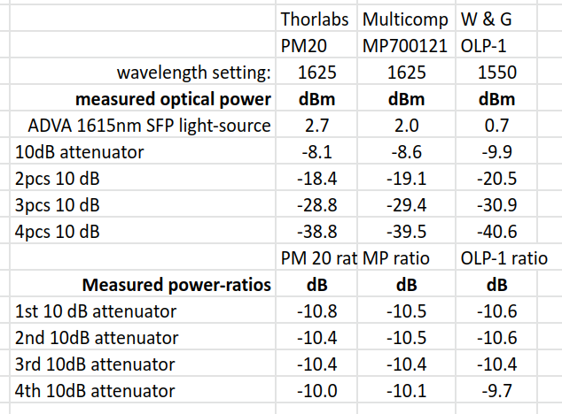
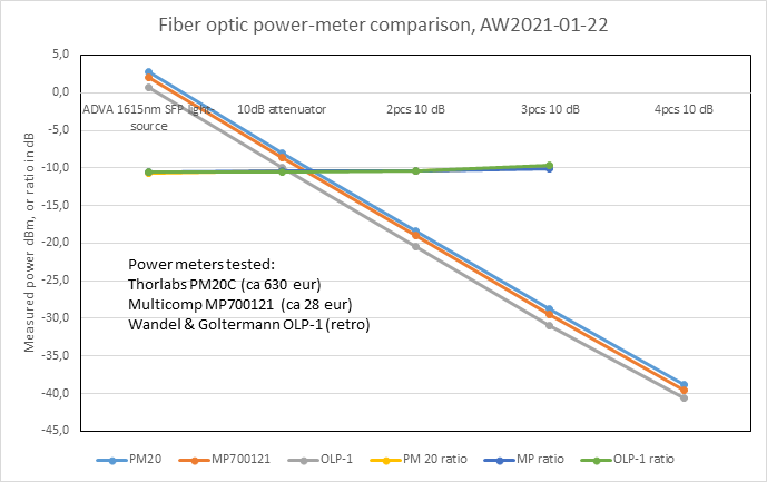
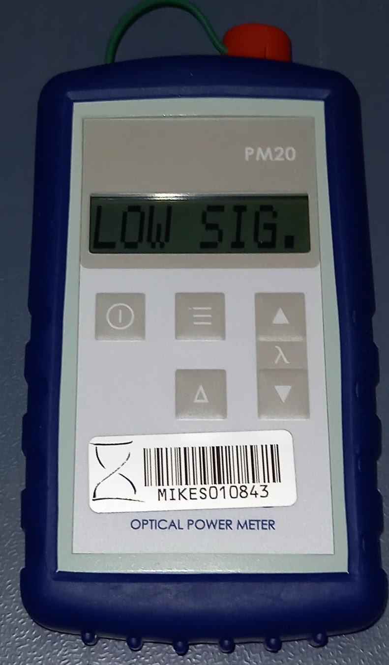
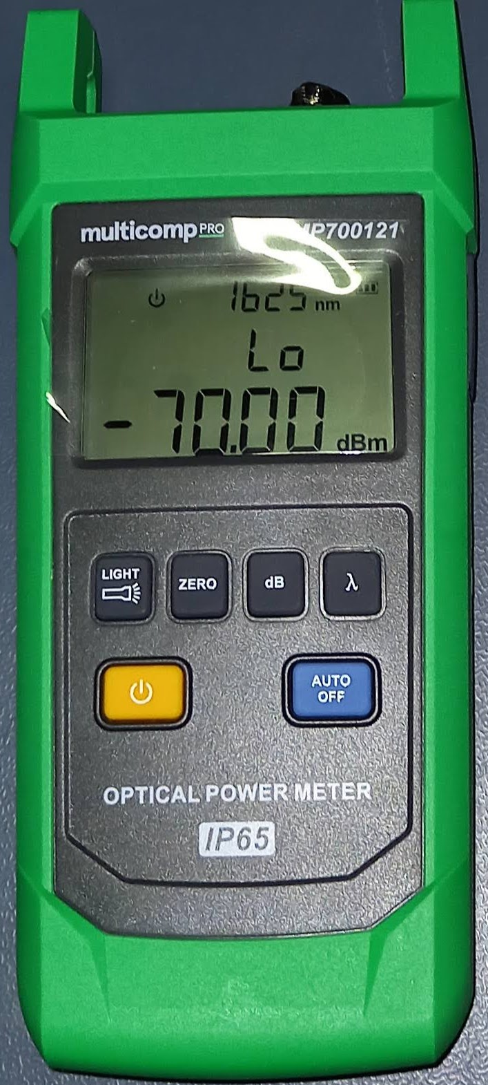
Fiber optic power meter test
Farnell is now selling a dirt-cheap (28 euros or so) Multicomp fiber optic power meter, so here's a quick comparison against other power meters in the lab.
It looks like the 28 euro meter performs good enough for most tasks in the lab. The Multicomp only has a few fixed wavelength settings, while the Thorlabs is adjustable in 1nm steps.

Fun with Chi-Squared
As mentioned before, the Chi-Squared inverse cumulative distribution is used when calculating confidence intervals in allantools.
When comparing computed confidence intervals against Stable32, there seems to be some systematic offsets, which I wanted to investigate.
While allantools uses scipy.stats.chi2.ppf(), It turns out that Stable32 uses an iterative method for EDF<=100, and an approximation from Abramowitz and Stegun: Handbook of Mathematical Functions for EDF>100. This 1964 book seems to be available online from many sites. The approximation (for large EDF) for the inverse chi-squared cumulative distribution is equations 26.4.17 (p410 in the PDF) (here nu is the equivalent degrees of freedom)
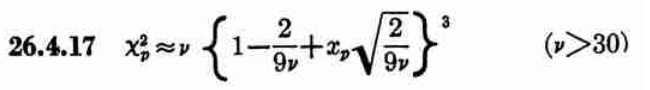
Where xp is from the inverse of the Normal cumulative distribution, computed via the approximation 26.2.22 (p404 in the PDF)
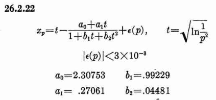
It also looks like the Stable32 source contains a misprint, where the a1 coefficient of 26.2.22 is used with two digits in the wrong order! (I did promise 'fun' in the title of this post!)
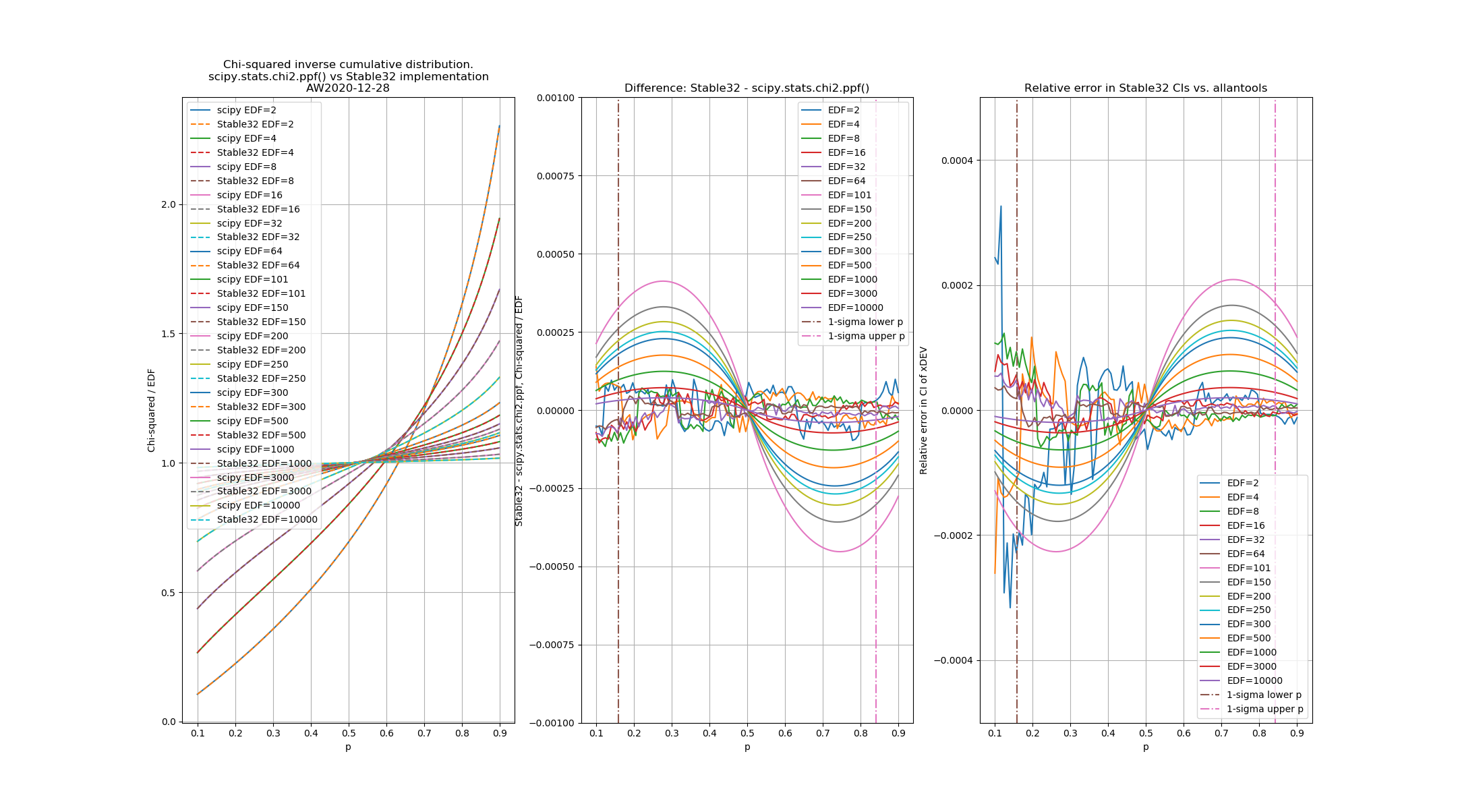
a1=0.27601 # typo in the Stable32 source code!? should be 0.27061If we plot both scipy.stats.chi2.ppf() and the Stable32 implementation for various EDF and probabilities we get the following:
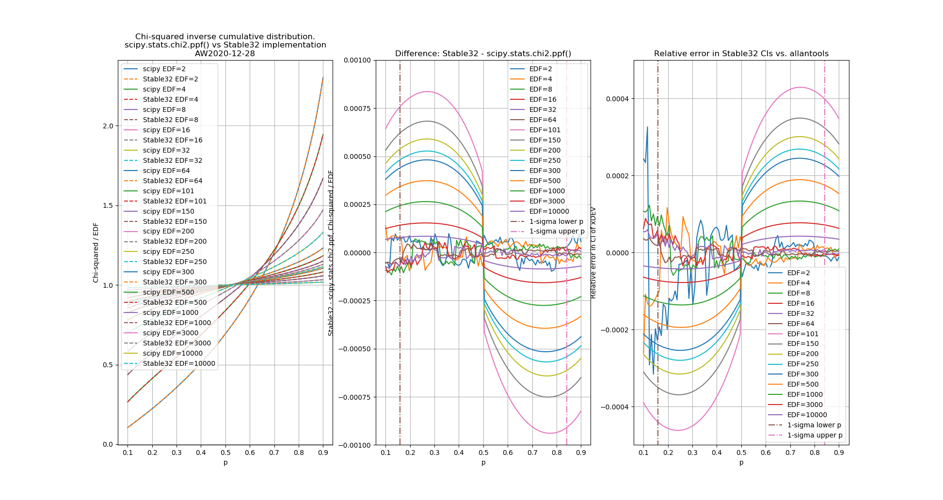
The leftmost figure shows Chi-Squared values (divided by EDF, to overlap all curves). There's not much difference between scipy and Stable32 visible at this scale. The middle figure shows the difference between the two algorithms. This shows very clearly the small (<100) EDF-region where the iterative algorithm in Stable32 produces a Chi-squared value in agreement with scipy to better than 4 digits (see the noisy traces around zero). This plot also reveals the shortcomings of the Abramovitz & Stegun approximation, together with the source-code misprint. The errors are largest, up to almost 1e-3 (in chi-squared/EDF) for EDF=101, and decrease with higher EDF. The rightmost figure shows what impact this has on computed confidence intervals - shown as relative errors. The confidence interval is proportional to sqrt(EDF/chi-squared). The dashed lines show the probabilities corresponding to 1-sigma confidence intervals, where we usually sample this function.
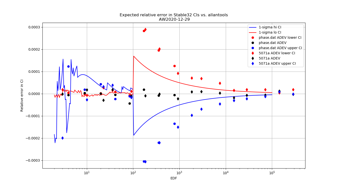
For 1-sigma confidence intervals we can now compare computed results with Stable32 and allantools to the comparison above of scipy and Abramovitz&Stegun + misprint.
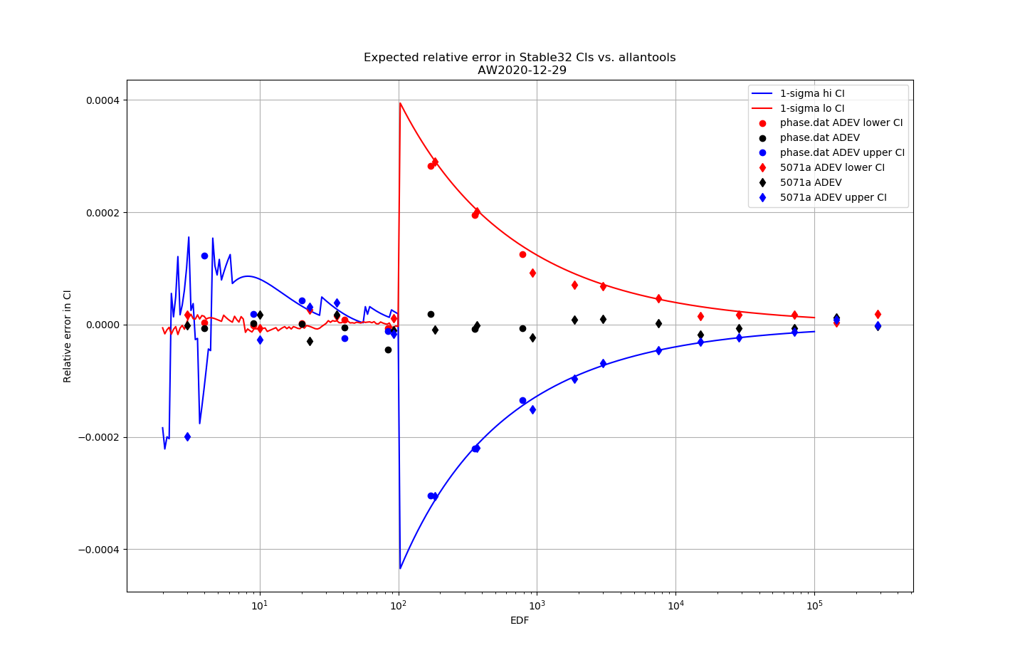
Are we having fun yet!? The comparison above between the two methods to compute the inverse chi-squared cumulative distribution seems to predict how Stable32 confidence intervals differ from allantools confidence intervals quite well! Note that Stable32 results are copy/pasted from the GUI with 5 significant digits, so some noise at the 1e-4 level is to be expected. Note that the relative error has a different sign depending on if we look at the lower or upper bound, and also depending on if we use the EDF<=100 iterative algorithm or the EDF>100 Abramovitz&Stegun+misprint approximation. For large EDF the upper bound (blue) of Stable32 is a bit too low, while the lower bound (red) is a bit too high.
Finally, the chi-squared figure and the expected confidence interval relative error figure, if we fix the misprint in the a1 coefficient:
Python code for producing these figures is available: chi2_stable32.py
The approximations used by Stable32 are not (yet?) included in allantools.
Second run of 88Sr+ optical clock
A second run of the optical clock on 2020-06-11 - this is a 64x speedup of the overnight live-stream:
88Sr+ clock first run
One of the very first runs of the servo-lock of our ultrastable clock-laser to the clock-transition at 445 THz in 88Sr+.
April Fools Ion
Despite the lockdown, some trapping in the lab this week. First single-ion experiments this year, after the 405 nm laser broke in January. Not much going on in these videos, but at least it's a single ion!
First clock-transition linewidth measurement give about a 200 Hz wide transition, so around 5e-13 fractionally.
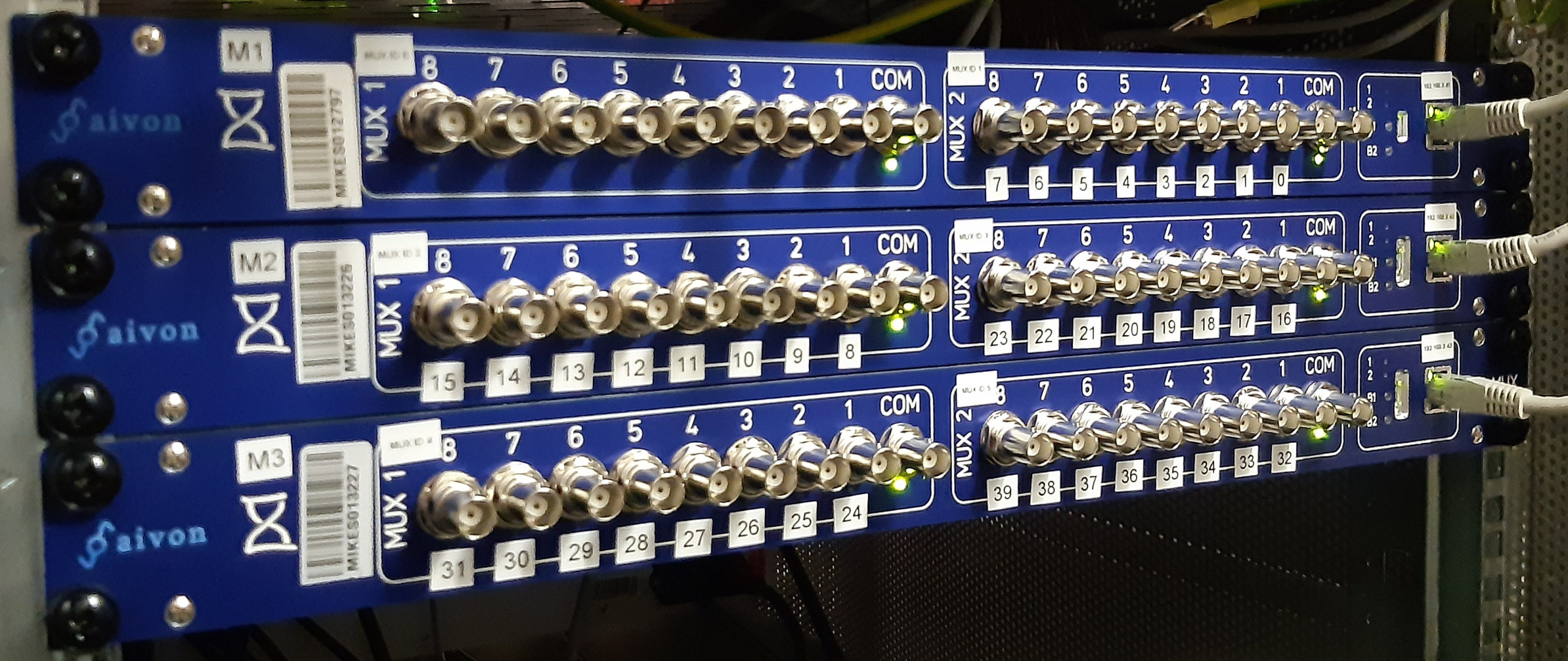
40-channel RF multiplexer
Just installed three of these 1U dual-1:8 RF-mutliplexers in the lab to make a 40-channel 1PPS measurement system. These are built by Aivon.
Time will tell how robust these are and if there are any failures in continuous use... Initial results from the field are good however.
We connect these in a depth-2 tree. One 1:8 mux is the top-level switch, with the remaining 5 providing 40 input-channels. This easily expands to 64 channels by adding one more 1U box. Beyond that I guess a depth-3 tree connection is required.
clock-transition scan at 128x speedup
Recorded at 2x speed with OBS from the youtube live-stream, then converted to MP4 with VLC, then run twice through Garmin Virb Edit producing 8x speedup both times.
88Sr+ clock transition in a low magnetic field
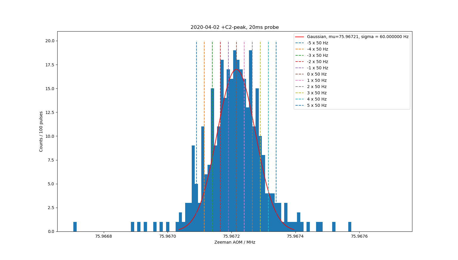
We've completed a second magnetic shielding layer, based on the same plywood+METGLAS concept as the first shield. This should further shield the 88Sr+ ion from unwanted magnetic field fluctuations. To further reduce the DC-field we've now applied a counter-field using a few milliAmps of current through three coils that surround the ion trap.
When the Zeeman components are this close together (the field is <0.4 uT) it is fairly quick to scan over the components. Here we see the four innermost pairs of peaks +/-C1 through +/-C4 of the clock-transition at 445 THz (674nm red light!). One scan runs in about one hour - and will be plotted on top of the older scans. We shoot 100 pulses of the laser-light at the ion and the height of the bar shows how many times we successfully drove the ion into the dark clock-state.
~800Hz wide clock-transition in 88Sr+
Here's the latest preliminary result from the VTT MIKES 88Sr+ ion clock (in case you missed the live-stream!):
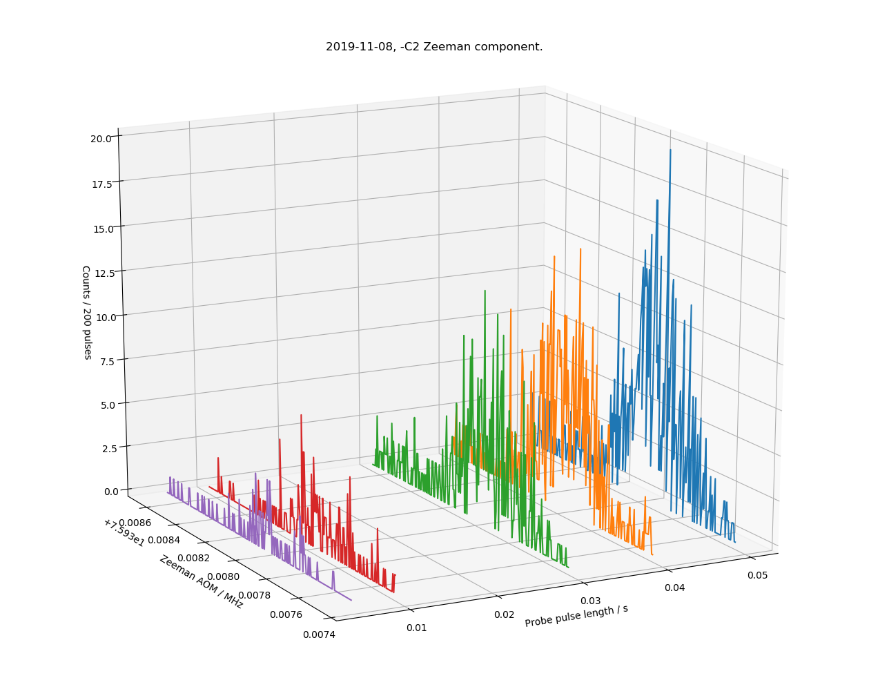
This shows a ~2 kHz slice (left axis, double the 1 kHz shown, because we plot the input frequency of a double-pass AOM) of the optical spectrum around 445 THz, where we expect to find the -C2 Zeeman component of the clock-transition in 88Sr+ (a secondary representation of the SI second). The right axis shows the probe-pulse length in seconds, where we see only a few percent excitation (z-axis) at short pulse lengths, but a clearer signal up to >10% at longer probe pulse lengths of 40 and 50 ms.
It ain't pretty, but considering the carrier is at 445 THz, this noisy and broad looking 800 Hz wide peak is still a measurement to a relative level of 2e-12. When fully operational a line-width of <10 Hz (2e-14) is expected.
Our experiment now has one metglas magnetic shield. This particular Zeeman component (-C2) has a sensitivity of 11 kHz/uT, so the observed linewidth of 800 Hz could be caused by a low-frequency AC magnetic field with an amplitude of 30-40 nT or so. We think the remaining DC-field is around 1.6 uT (down from 66 uT without the metglas shield).
Among other improvements, next is building a second metglas shield, to reduce AC fluctuations in the magnetic shield even further. Stay tuned...