Sliptonic has worked on connecting FreeCAD with OpenVoronoi to produce V-carving (aka medial-axis) toolpaths.
I worked on the OpenVoronoi stuff 7 years ago and we made this video back then:
Sliptonic has worked on connecting FreeCAD with OpenVoronoi to produce V-carving (aka medial-axis) toolpaths.
I worked on the OpenVoronoi stuff 7 years ago and we made this video back then:
Kasuyasu Hamada has made a lot of progress with my earlier cutsim work. Code is on github: https://github.com/KASUYASU/cutsim
For a historical time-line see the cutsim tag.
The basic CAM-algorithm called axial tool projection, or drop-cutter, works by dropping down a cutter along the z-axis, at a chosen (x,y) location, until we make contact with the CAD model. Since the CAD model consists of triangles, drop-cutter reduces to testing cutters against the triangle vertices, edges, and facets. The most advanced of the basic cutter shapes is the BullCutter, a.k.a. Toroidal cutter, a.k.a. Filleted endmill. On the other hand the most involved of the triangle-tests is the edge test. We thus conclude that the most complex code by far in drop-cutter is the torus edge test.
The opencamlib code that implements this is spread among a few files:
The special cases where we contact the flat bottom of the cutter, or the cylindrical shaft, are easy to deal with. So in the general case where we make contact with the toroid the geometry looks like this:
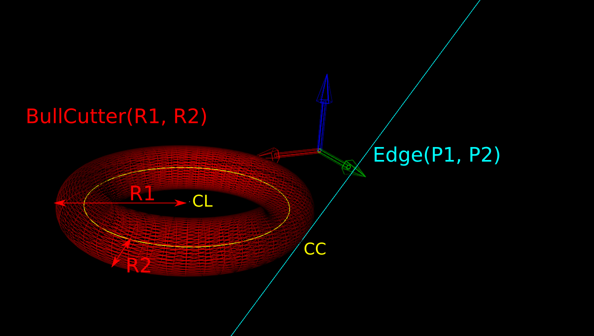
Here we've fixed the XY coordinates of the cutter location (CL) point, and we're using a filleted endmill of radius R1 with a corner radius of R2. In other words R1-R2 is the major radius and R2 is the minor radius of the Torus. The edge we are testing against is defined by two points P1 and P2 (not shown). The location of these points doesn't really matter, as we do the test against an infinite line through the points (at the end we check if CC is inside the P1-P2 edge). The z-coordinate of CL is the unknown we are after, and we also want the cutter contact point (CC).
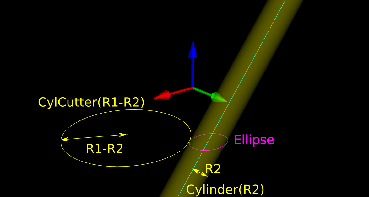
There are many ways to solve this problem, but one is based on the offset ellipse. We first realize that dropping down an R2-minor-radius Torus against a zero-radius thin line is actually equivalent to dropping down a zero-minor-radius Torus (a circle or 'ring' or CylCutter) against a R2-radius edge (the edge expanded to an R2-radius cylinder). If we now move into the 2D XY plane of this circle and slice the R2-radius cylinder we get an ellipse:
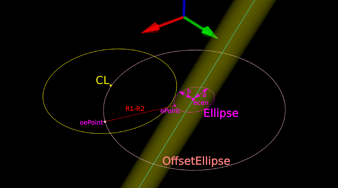
The circle and ellipse share a common virtual cutter contact point (VCC). At this point the tangents of both curves match, and since the point lies on the R1-R2 circle its distance to CL is exactly R1-R2. In order to find VCC we choose a point along the perimeter of the ellipse (an ellipse-point or ePoint), find out the normal direction, and go a distance R1-R2 along the normal. We arrive at an offset-ellipse point (oePoint), and if we slide the ePoint around the ellipse, the oePoint traces out an offset ellipse.
Now for the shocking news: an offset-ellipse doesn't have any mathematically convenient representation that helps us solve this!
Instead we must numerically find the best ePoint such that the oePoint coincides with CL. Like so:
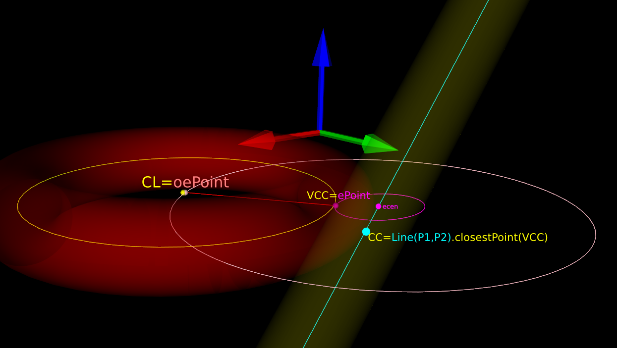
Once we've found the correct ePoint, this locates the ellipse along the edge and the Z-axis - and thus CL and the cutter . If we go back to looking at the Torus it is obvious that the real CC point is now the point on the P1-P2 line that is closest to VCC.
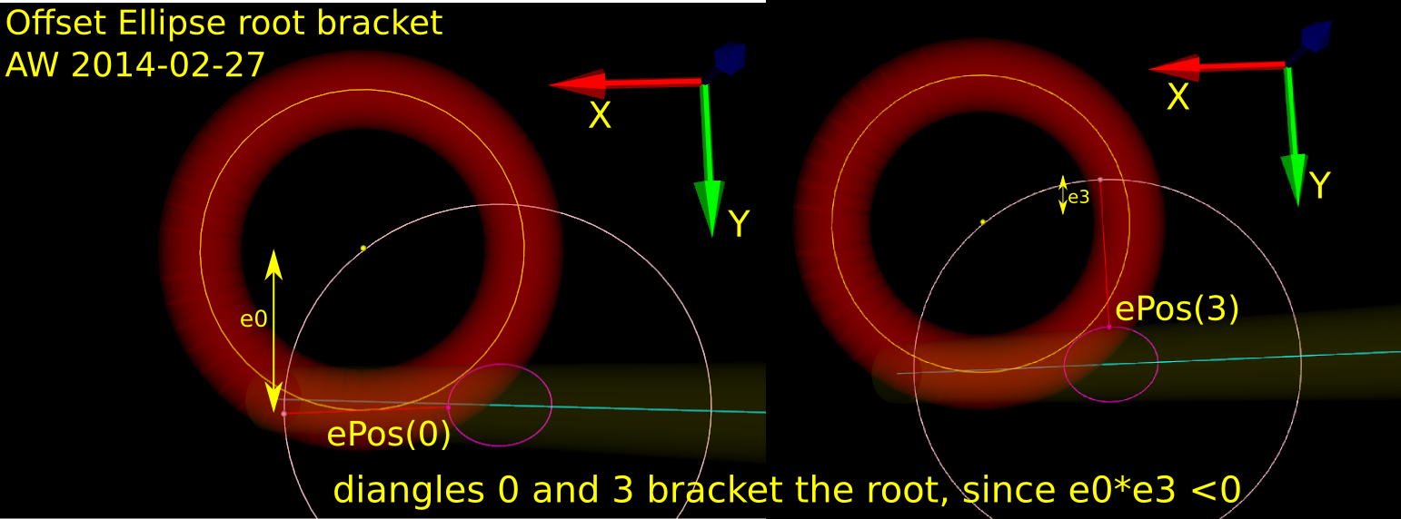
In order to run Brent's root finding algorithm we must first bracket the root. The error we are minimizing is the difference in Y-coordinate between the oePoint and the CL point. It turns out that oePoints calculated for diangles of 0 and 3 bracket the root. Diangle 0 corresponds to the offset normal aligned with the X-axis, and diangle 3 to the offset normal aligned with the Y-axis:
Finally a clarifying drawing in 2D. The ellipse center is constrained to lie on the edge, which is aligned with the X-axis, and thus we know the Y-coordinate of the ellipse center. What we get out of the 2D computation is actually the X-coordinate of the ellipse center. In fact we get two solutions, because there are two ePoints that match our requirement that the oePoint should coincide with CL:
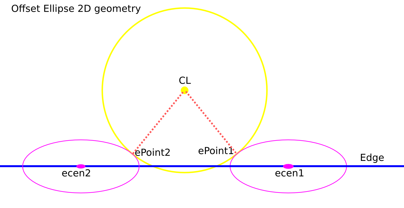
Once the ellipse center is known in the XY plane, we can project onto the Edge and find the Z-coordinate. In drop-cutter we obviously approach everything from above, so between the two potential solutions we choose the one with a higher z-coordinate.
The two ePoint solutions have a geometric meaning. One corresponds to a contact between the Torus and the Edge on the underside of the Torus, while the other solution corresponds to a contact point on the topside of the Torus:
I wonder how this is done in the recently released pycam++?
There might be renewed hope for a FreeCAD CAM module. Here are some examples of what opencamlib and openvoronoi can do currently.
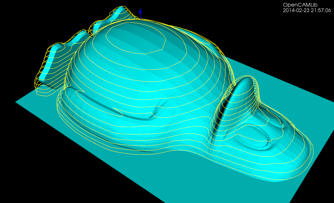
The drop-cutter algorithm is the oldest and most stable. This shows a parallel finish toolpath but many variations are possible.
The waterline algorithm has some bugs that show up now and then, but mostly it works. This is useful for finish milling of steep areas for the model. A smart algorithm would use paralllel finish on flat areas and waterline finish on steep areas. Another use for the waterline algorithm is "terrace roughing" where the waterline defines a pocket at a certain z-height of the model, and we run a pocketing path to rough mill the stock at this z-height. Not implemented yet but doable.
This shows offsets calculated with openvoronoi. The VD algorithm is fairly stable for input geometries with line-segments, but some corner cases still cause problems. It would be nice to have arc-segments as input also, but this requires additional work.
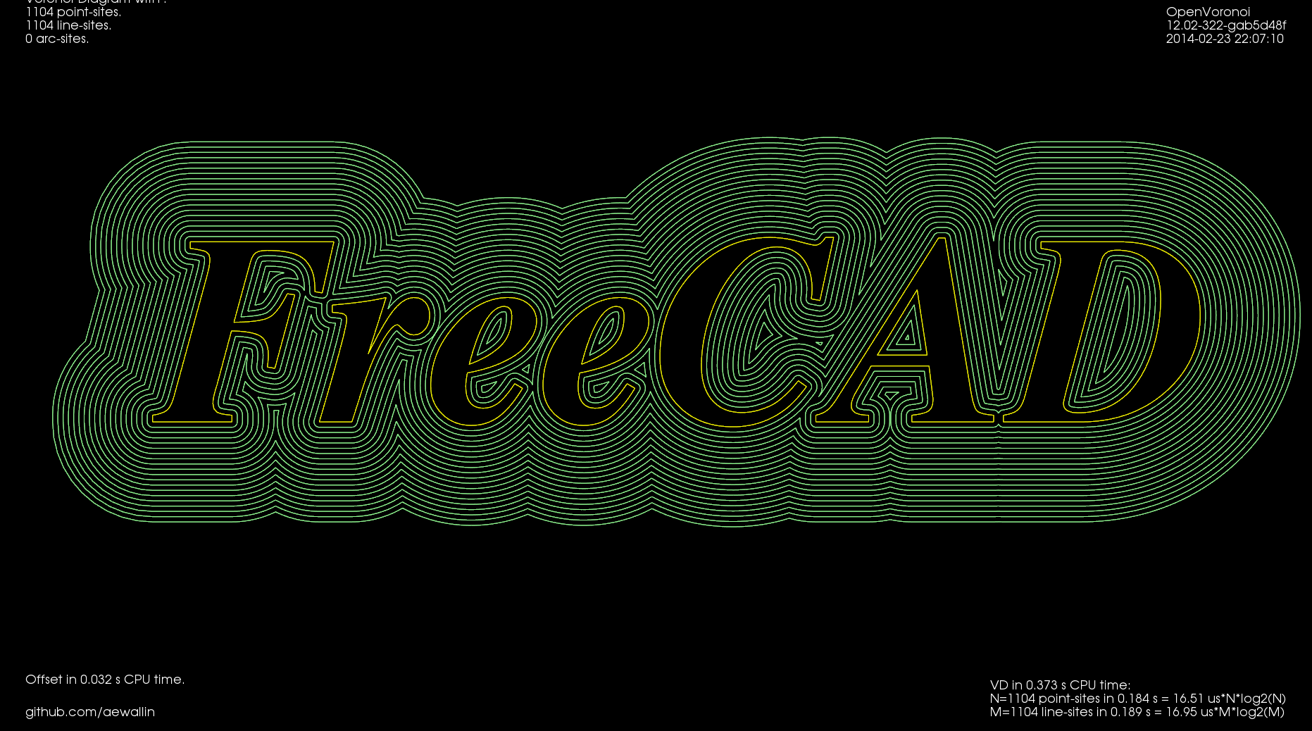
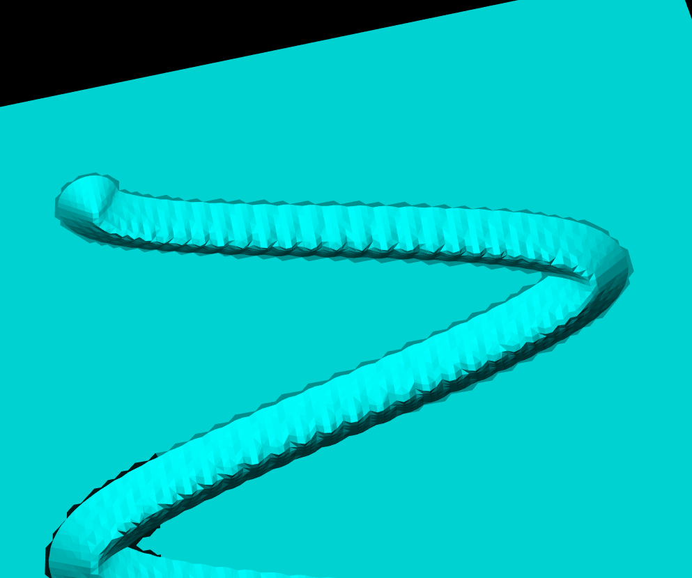
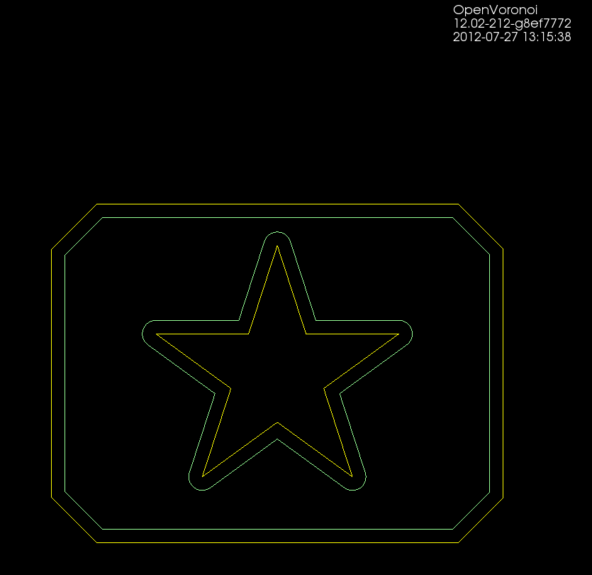
The VD is easily filtered down to a medial-axis, more well-known as a V-carving toolpath. I've demonstrated this for a 90-degree V-cutter, but toolpath is easy to adapt for other angles. Input geometry comes from truetype-tracer (which in turn uses FreeType).

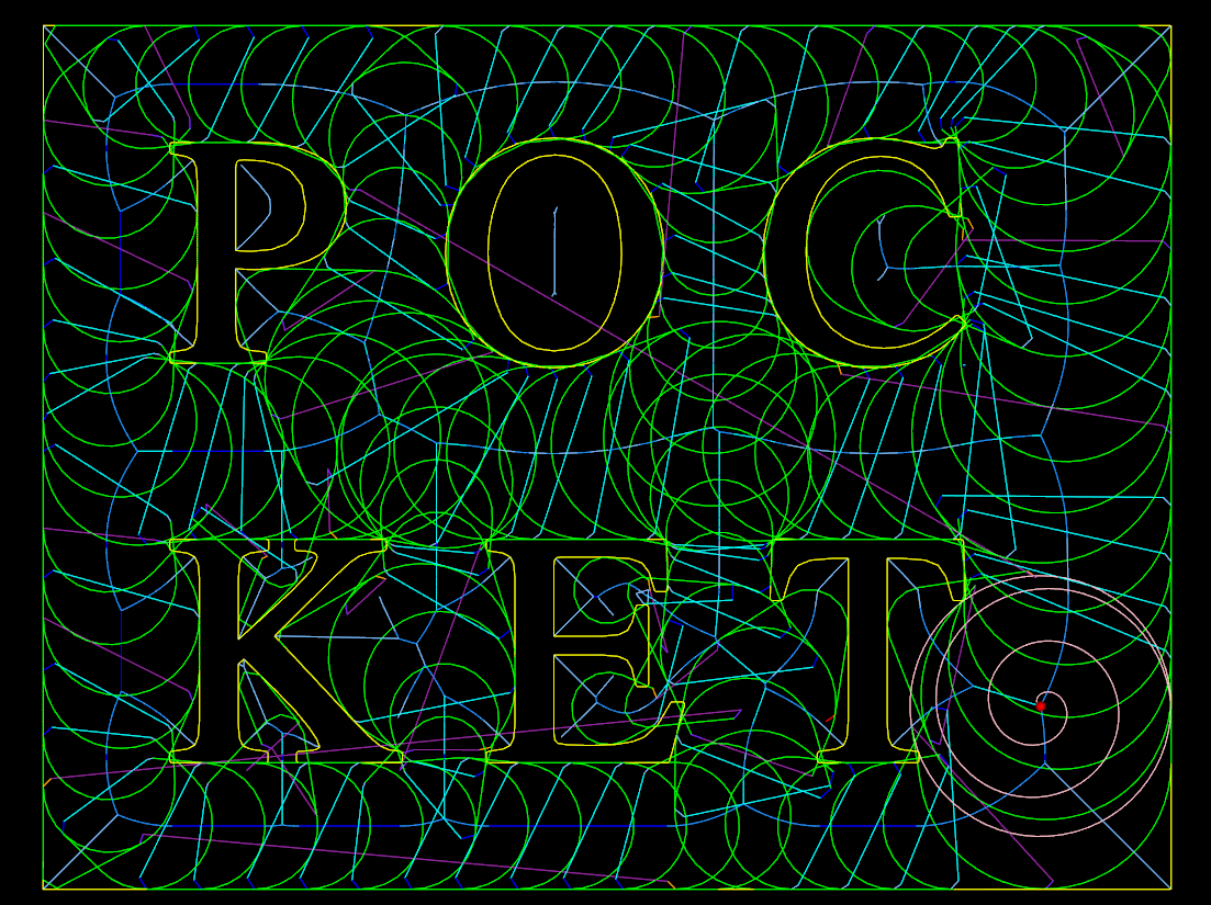
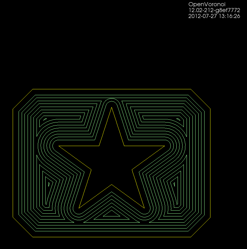
Finally there is an experimental advanced pocketing algorithm which I call medial-axis-pocketing. This is just a demonstration for now, but could be developed into an "adaptive" pocketing algorithm. These are the norm now in modern CAM packages and the idea is not to overload the cutter in corners or elsewhere - take multiple light passes instead.
The real fun starts when we start composing new toolpath strategies consisting of many of these simple/basic ones. One can imagine first terrace-roughing a part using the medial-axis-pocketing strategy, then a semi-finish path using a smart shallow/steep waterline/parallel-finish algorithm, and finally a finish operation or even pencil-milling.
Dual contouring uses a quadratic-error-function (QEF) to position a vertex inside each octree-node (cube) where the implicit distance-field that defines our geometry changes sign. The vertex is positioned so that the QEF is minimized. This allows for an octree simplification strategy where we combine all the QEFs of the eight child-nodes, and see if we can replace the eight vertices they define with with a single vertex one level up in the octree.
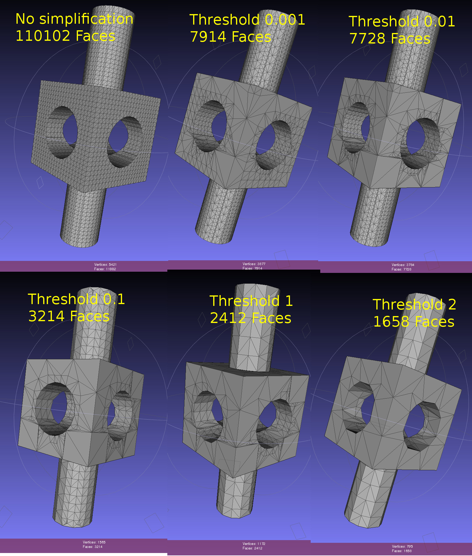
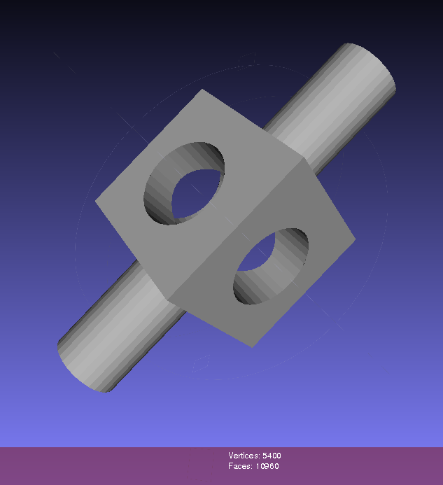
This image shows the dual contouring code run on the same input data with various levels of simplification. Even a small threshold value of 0.001 reduces the number of triangles more than ten-fold. Too large a threshold produces jagged edges. Note that dual contouring of the original dataset where each leaf-node is at the same (maximal) depth of the tree produces only quad polygon output. When we simplify and collapse some nodes to non-maximal depth the algorithm also produces triangles - where a collapsed node is adjacent to nodes deeper in the tree.
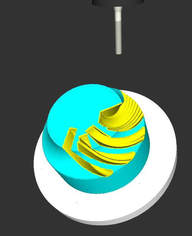
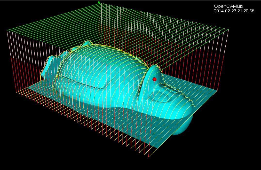
Here's an image from the CNC-milling simulator I am working on. It stores a signed distance field in an adaptively subdivided octree. To render a surface of the stock we then run an isosurface extraction algorithm. The most well-known of these is the Marching Cubes (MC) algorithm, used here also. One problem with MC is that it doesn't preserve fine detail (like sharp edges) very well, and many times there are also gaps or cracks in the surface. Both of these problems are visible below.
From about 2000 onward there are a number of papers that try to improve on MC. The most promising seems to be Dual Contouring, by Tao Ju. There is both c++ and Java LGPL code for DC on sourceforge, and I made some slight changes to make it compile with cmake on Ubuntu: https://github.com/aewallin/dualcontouring
The output PLY file can be viewed with meshlab:
So far so good. Now the task is to either rewrite my octree + boolean CSG operations code to use the data structure used in the DC code, or vice versa, change the DC code to use my datastructure.
Some basic pocketing loops generated on the train today.
Using pycam's revise_directions() function it is possible to clean up the DXF data and classify polygons into pockets and islands.
There's a new parameter N_offsets
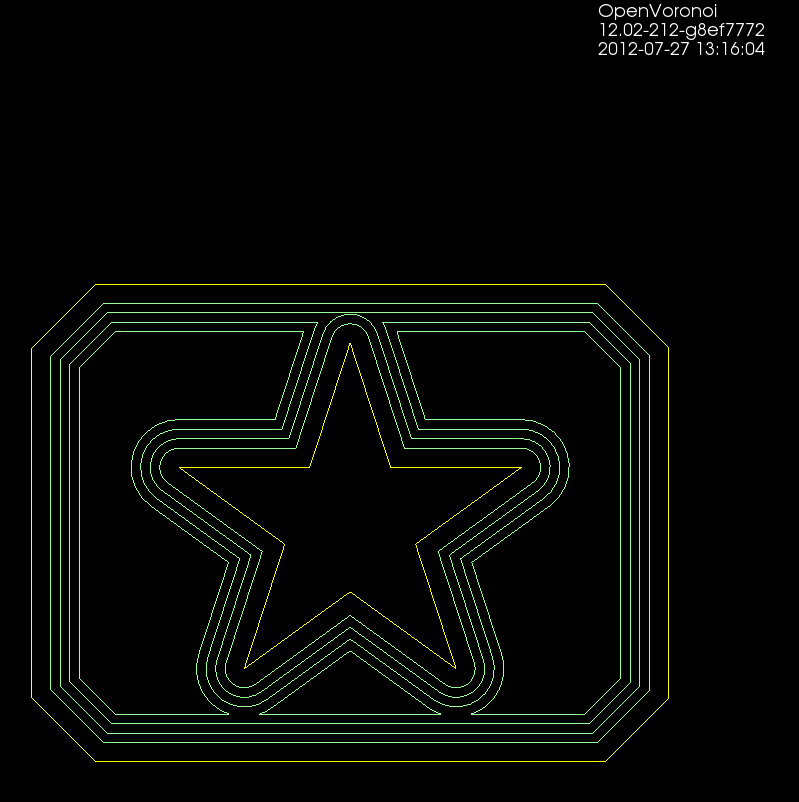
N_offsets=1 generates just a single offset at a specified offset-distance.N_offsets=2... generates the specified number of offsets. Possibly with an increment in offset-distance that is not equal to the initial offset-distance. This happens e.g. when we want the final pass of the tool to be one cutter-radius from the input geometry but the material is difficult to machine and we want the "step-over" for interior offset-loops to be less than the cutter-radius.N_offsets=-1 produces a complete interior pocketing path. Offsets are first generated at the initial offset distance and successive offsets are then generated at increasing offset distance until no offset-output is generated.
Todo: Nesting, Linking, Optimization.
There's no nesting among the loops here. The algorithm will have no clue in what order to machine the offset loops. A naive approach is to machine all loops at the maximum offset distance, then move one loop outwards, etc. But this is clearly not good as the tool would jump between the growing pockets during machining. Nesting information should be straightforward to extract from the voronoi diagram during offset-generation. The nested loops form a tree/graph, which we traverse in some suitable order to machine the entire pocket.
Also, there is no linking of these loops to eachother. For a machining toolpath one wants to link the offsets to each other so that the tool can be kept down in the material when we move from one offset loop to the next. A simple algorithm for linking should be straightforward, but I suspect something more involved is required to prevent overcutting with sufficiently complex input geometry.
When one has nested and linked offset paths, in general there still will remain "pen-up", "rapid traverse", "pen down" transitions. An asymmetric TSP solver could be run on this to minimize the rapid traverse distance (machining time).
A very early result with trying to use openvoronoi from pycam:

Pycam reads the geometry from a DXF file, does some pre-processing of the geometry, pushes it over to openvoronoi which computes a VD and the offsets. Offsets (line-segments and arcs) are then communicated back to pycam for display and g-code generation.
Here's some benchmark data for constructing the Voronoi diagram (or its dual, the Delaunay triangulation) for random point sites. Code for this benchmark is over here: https://github.com/aewallin/voronoi-benchmark

OpenVoronoi is my own effort using the incremental topology-oriented algorithm of Sugihara&Iri and Held. Floating-point coordinates with all sites falling within the unit-circle are used. Fast double-precision arithmetic is used for geometric predicates (e.g. "in-circle") during the incremental construction of the diagram, since the topology-oriented approach ensures that the algorithm finishes and produces an output graph regardless of errors in the geometric predicates. Quad-precision arithmetic is used for positioning vd-vertices. This benchmark runs in ca 7us*N*log2(N) time.
Boost.Polygon uses Fortune's sweepline algorithm. Only integer input coordinates are allowed, which ensures that geometric predicates can be computed exactly. Lazy arithmetic, where a high-precision slower number-type is used only when required, is used. This benchmark runs in ca 0.2us*N*log2(N) time.
CGAL uses exact geometric computation, which is slow but supposedly robust. The run-time gets worse with increasing problem-size and doesn't seem to fall on an O(N*log(N)) line.
Some thoughts:
I started working on arc-sites for OpenVoronoi. The first things required are an in_region(p) predicate and an apex_point(p) function. It is best to rapidly try out and visualize things in python/VTK first, before committing to slower coding and design in c++.
in_region(p) returns true if point p is inside the cone-of-influence of the arc site. Here the arc is defined by its start-point p1, end-point p2, center c, and a direction flag cw for indicating cw or ccw direction. This code will only work for arcs smaller than 180 degrees.
def arc_in_region(p1,p2,c,cw,p): if cw: return p.is_right(c,p1) and (not p.is_right(c,p2)) else: return (not p.is_right(c,p1)) and p.is_right(c,p2) |

Here randomly chosen points are shown green if they are in-region and pink if they are not.
apex_point(p) returns the closest point to p on the arc. When p is not in the cone-of-influence either the start- or end-point of the arc is returned. This is useful in OpenVoronoi for calculating the minimum distance from p to any point on the arc-site, since this is given by (p-apex_point(p)).norm().
def closer_endpoint(p1,p2,p): if (p1-p).norm() < (p2-p).norm(): return p1 else: return p2 def projection_point(p1,p2,c1,cw,p): if p==c1: return p1 else: n = (p-c1) n.normalize() return c1 + (p1-c1).norm()*n def apex_point(p1,p2,c1,cw,p): if arc_in_region(p1,p2,c1,cw,p): return projection_point(p1,p2,c1,cw,p) else: return closer_endpoint(p1,p2,p) |

Here a line from a randomly chosen point p to its apex_point(p) has been drawn. Either the start- or end-point of the arc is the closest point to out-of-region points (pink), while a radially projected point on the arc-site is closest to in-region points (green).
The next thing required are working edge-parametrizations for the new type of voronoi-edges that will occur when we have arc-sites (arc/point, arc/line, and arc/arc).