waterline – anderswallin.net

Comparing waterlines

Here's a picture which compares the waterline toolpath for different cutters around a single triangle (cyan). The outermost path (red) is for a cylindrical cutter where we always make contact with either the shaft of the cutter or the circular rim/end of the cutter. Next is the yellow line for the toroidal or BullCutter, followed by the green line for a spherical or BallCutter. The innermost waterline (pink) is for a conical ConeCutter.

Here are some more waterlines at different heights. This exercise has uncovered at least two new bugs with CylCutter and ConeCutter! The CylCutter seems to fail when asking for a waterline at z=0.0, so that might hint at where the problem is. I'm not sure what is causing the jagged shape with ConeCutter.

Update: The cl-points for conecutter look right, so there must be something strange going on with the weave??

Cone-cutter waterlines

I'm not sure why it has taken so long to get the push-cutter methods for ConeCutter written. You would think that the cylindrical, spherical, or toroidal cases are at least as hard. Somehow I have just avoided working on the cone-cutter...

The easy part is as usual contacts between the cutter and the vertices of a triangle - these are shown as red dots. Contact with the facet of the triangle can be made in two ways (1) by the tip of the cone, or (2) by the circular base of the cone, when the facet is steeper than the cone. These are shown in green.

The more involved case is contacts with the edge of the triangle. There are again two cases: We can make contact with the circular base of the cone (cyan dots), or we can make contact with the actual conical part of the cutter (pink dots).

Here is an animation that gives the code a workout. Note how the color of the contact-points changes depending both on what part of the triangle we are making contact with and on what part of the cutter is making the contact.

I have now used github for a while, and will probably merge the conecutter feature-branch into master very soon. Almost as soon as I tried github google-code also started supporting git, but possibly the forking and social aspects of github make a switch worthwhile anyway.

There are some interesting developments on the higher level Waterline/Weave algorithm also, which will reduce the memory-consumption of the algorithm from N*N to N+N (where N is the number of Fibers). This will hopefully make Waterline more useful as now many people have been running out of RAM or just seen sudden crashes. Stay tuned...

Weave notes

As noted before, the waterline operation consists of radial cutter projection ("push cutter") along fibers/dexels, followed by a weave/grid construction, and contouring to produce the final toolpath. Like so:

The new Weave2 class builds up a half-edge diagram in a smart way, maintaining "next" and "previous" pointers for each edge, so that the green toolpath loop can easily be found by traversing from one CL-point to the next simply following the "next" pointer:

(The magenta arrows are "next" pointers which point from one edge to the next)

The main part of the algorithm looks at one X-fiber (from xL to xU) and one Y-fiber (from yL to yU) at a time and inserts a new internal vertex (v) into the diagram, while maintaining the existing "next" and "prev" pointers.

I didn't come up with any elegant object-oriented scheme that would do this nicely, so the build() function in the code just peeks and pokes and updates all of the 24 pointers in a brute-force kind of style.

I suspect that the O(n^2) time-complexity is optimal, since with n X-fibers and n Y-fibers there will be roughly n*ninternal vertices in the grid, and they all have to be processed (?unless we can prune the grid and ignore internal areas and focus on the edge of the weave?).

Faster Waterline

I've written a new Weave class for opencamlib which makes the waterline operation faster.

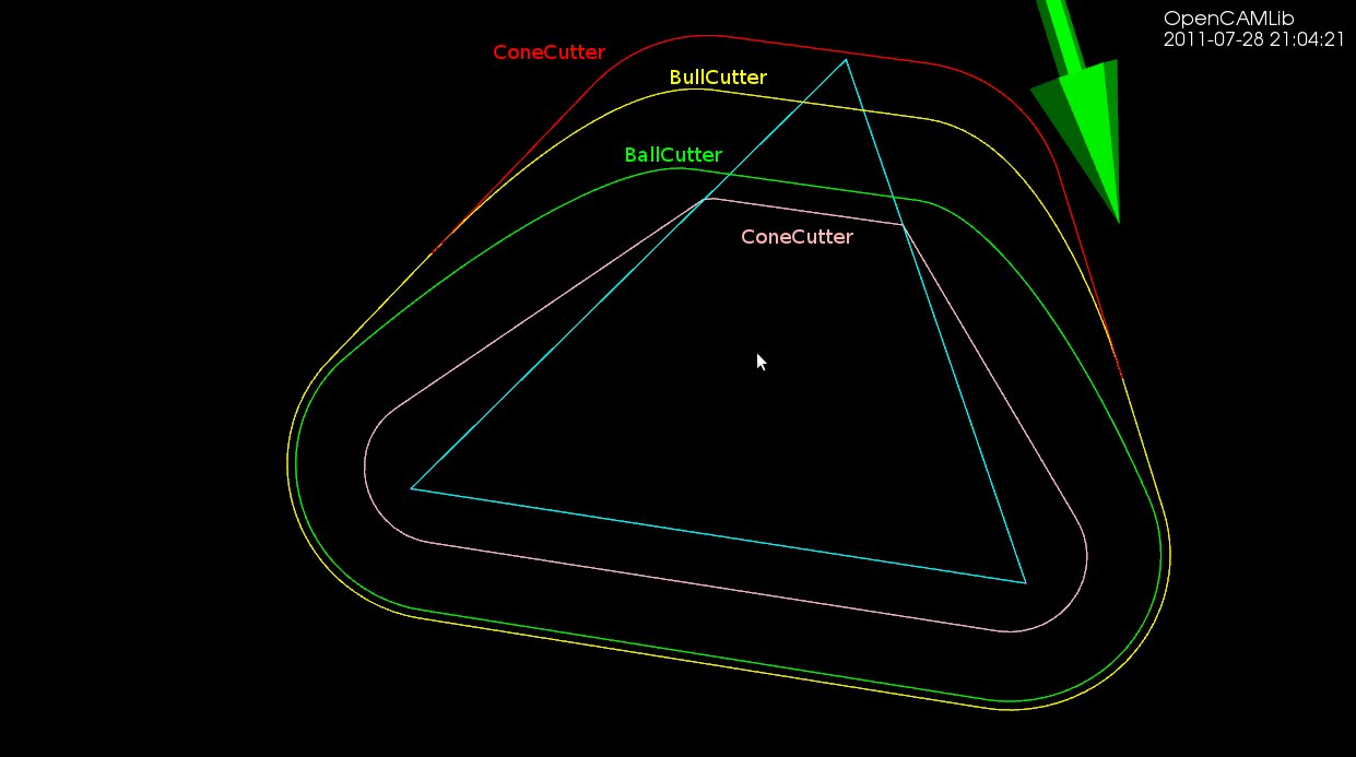
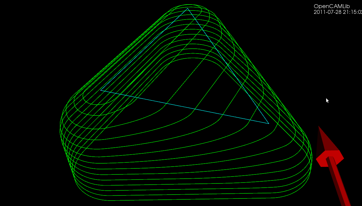
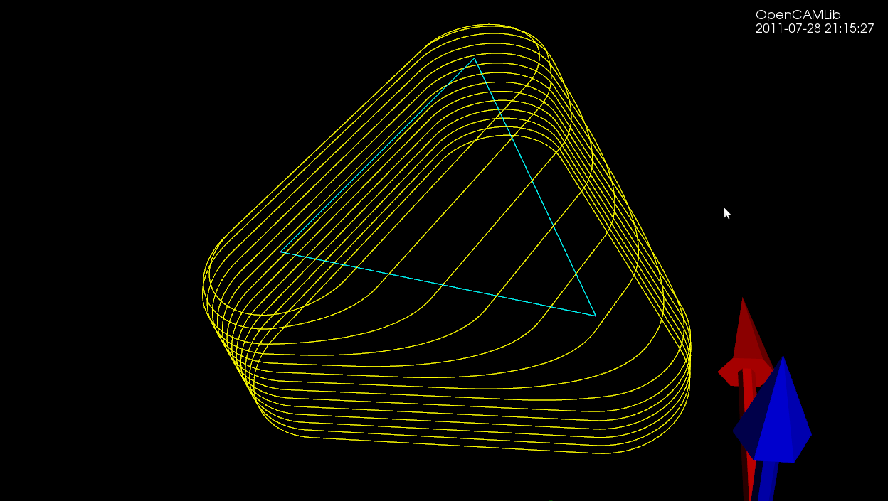
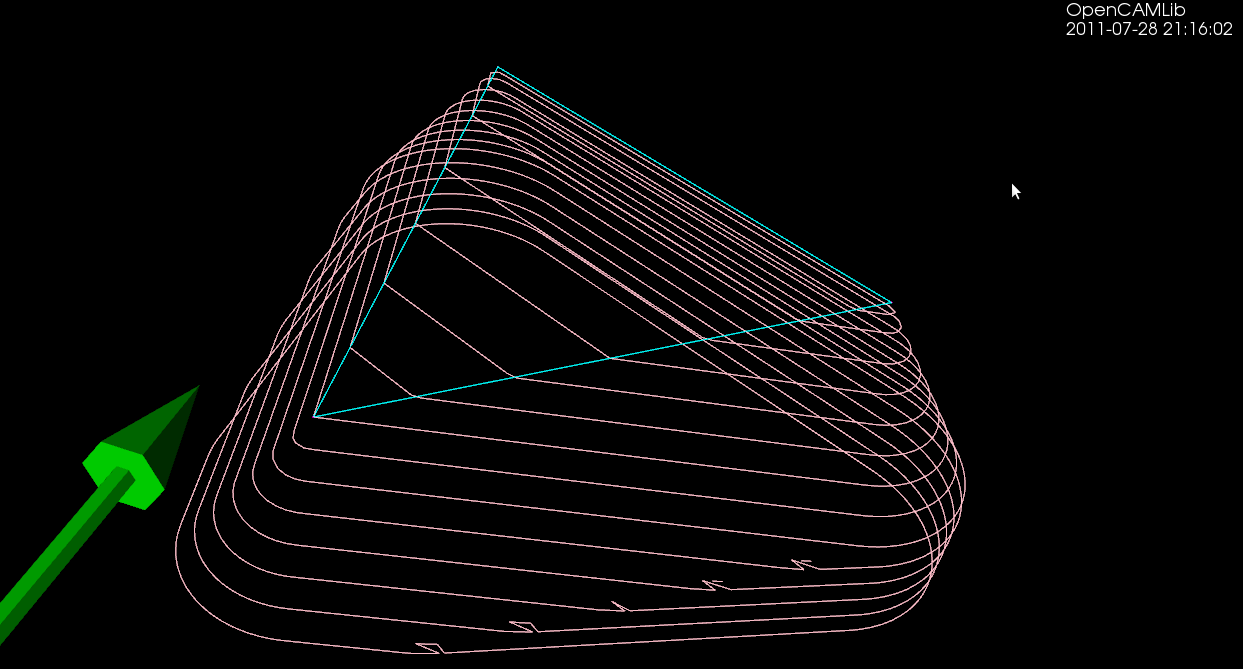
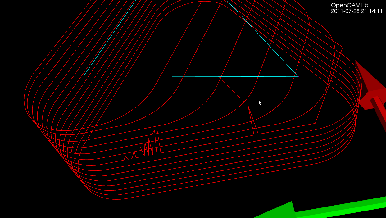
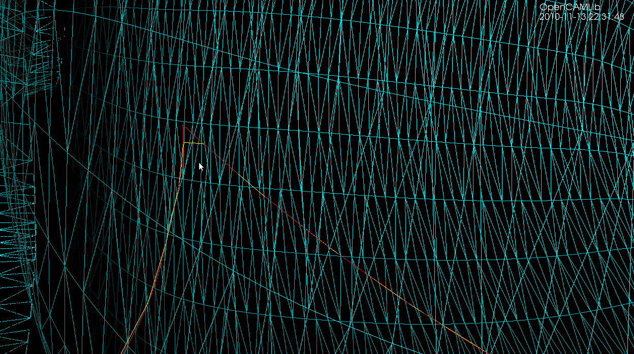
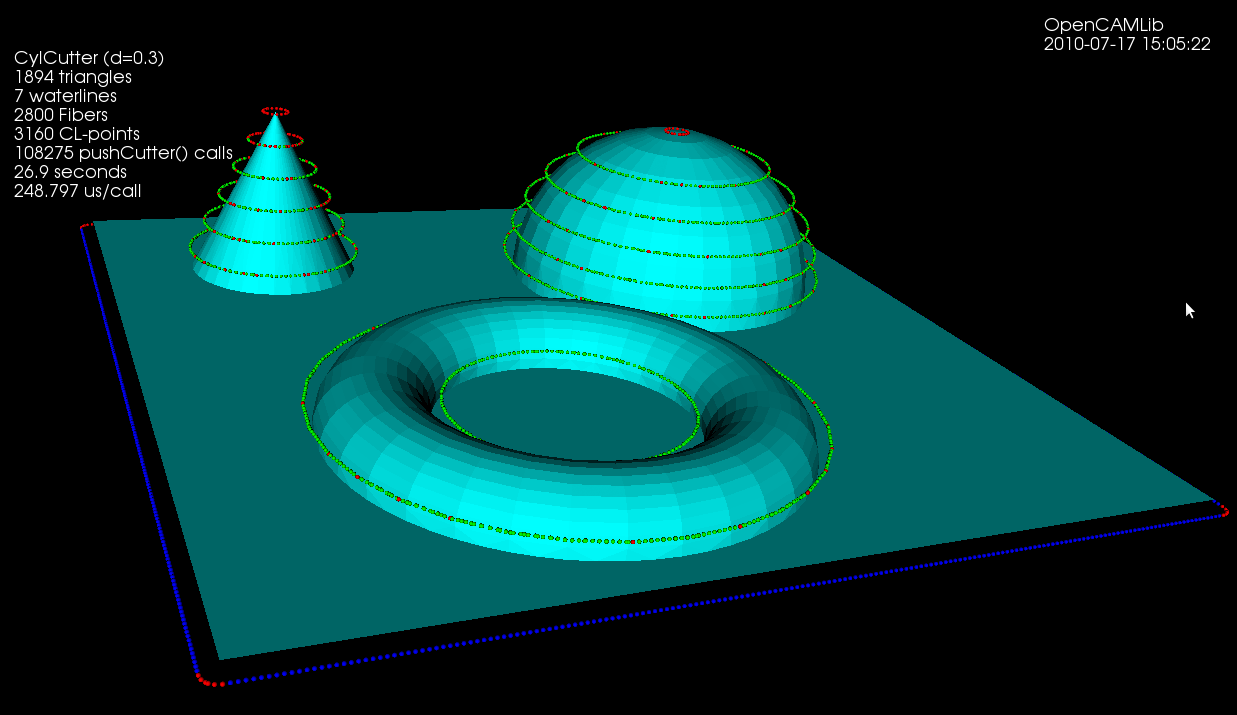
The first test-case is a single triangle, and we calculate a number of waterlines at different z-heights using a ball-cutter:

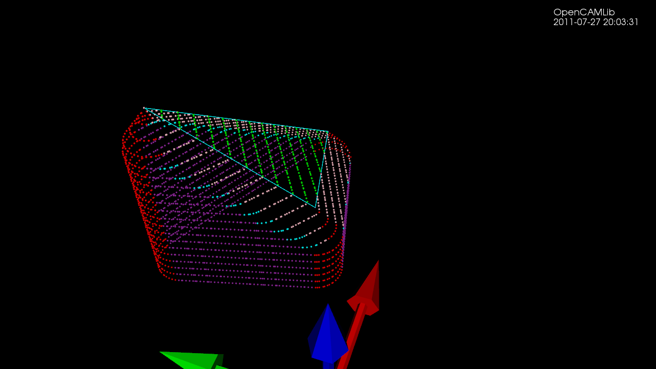
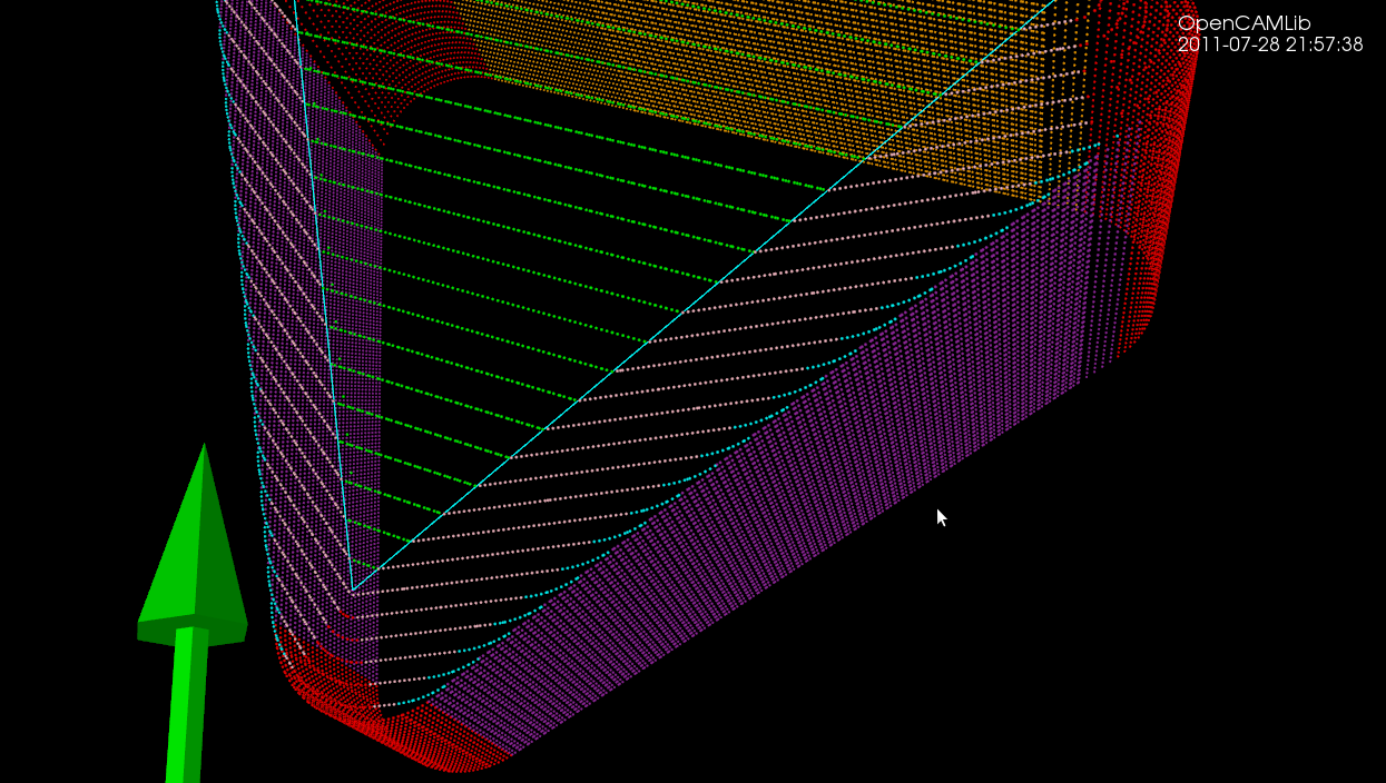
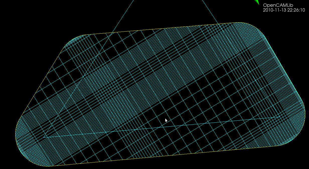
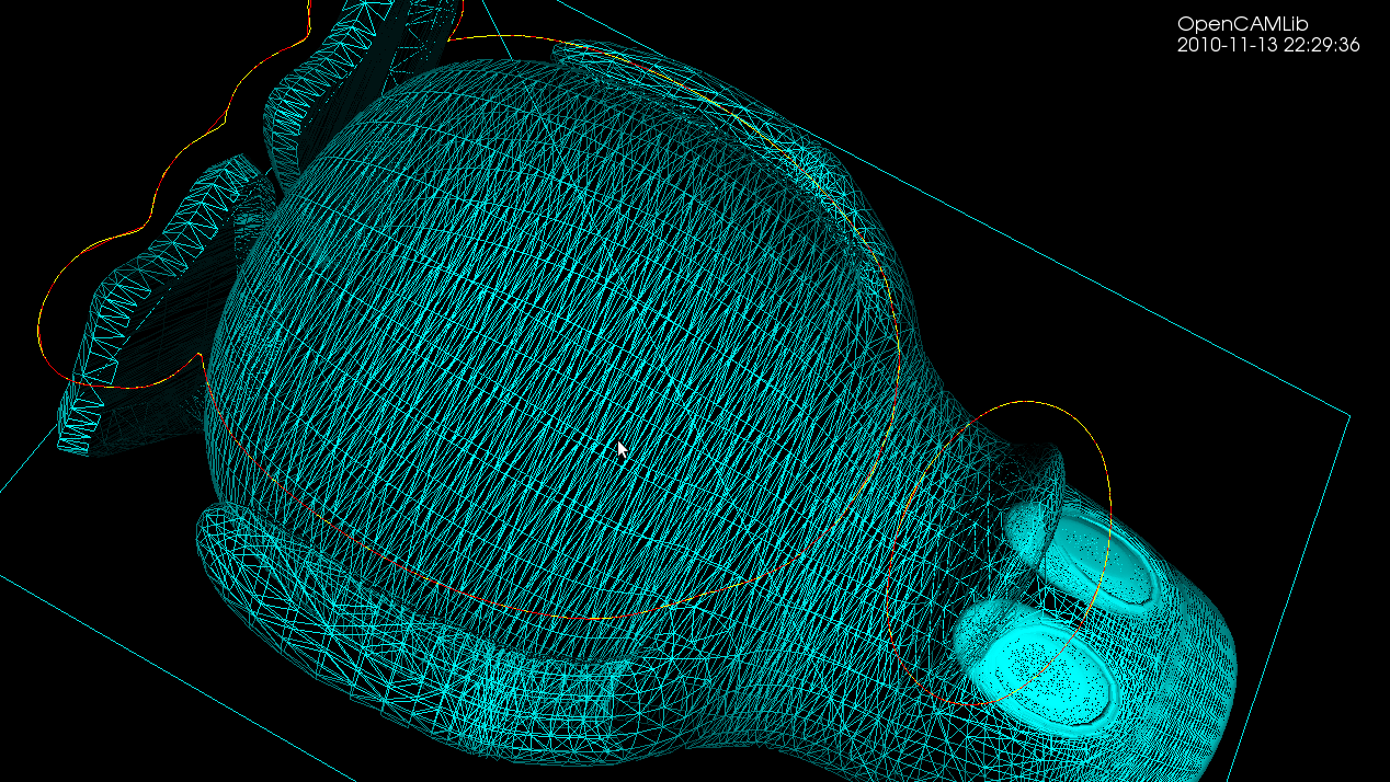
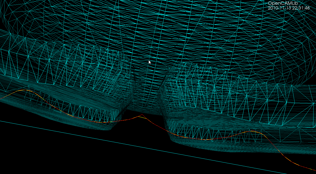
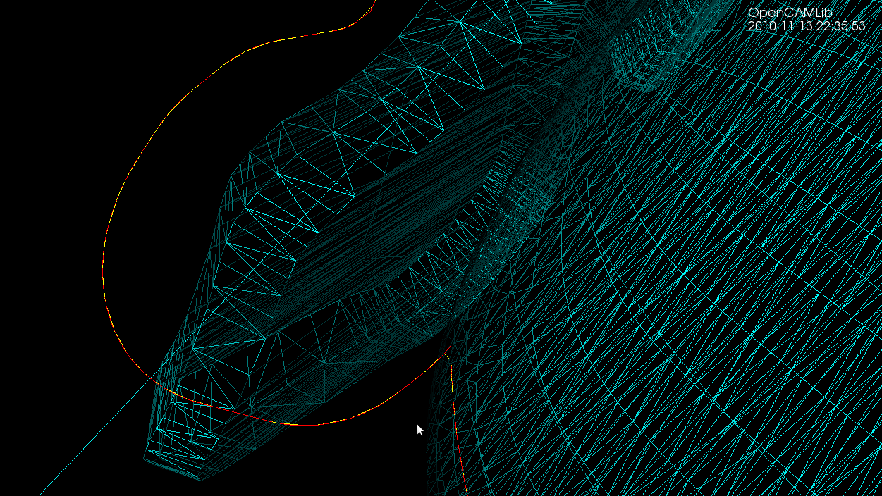
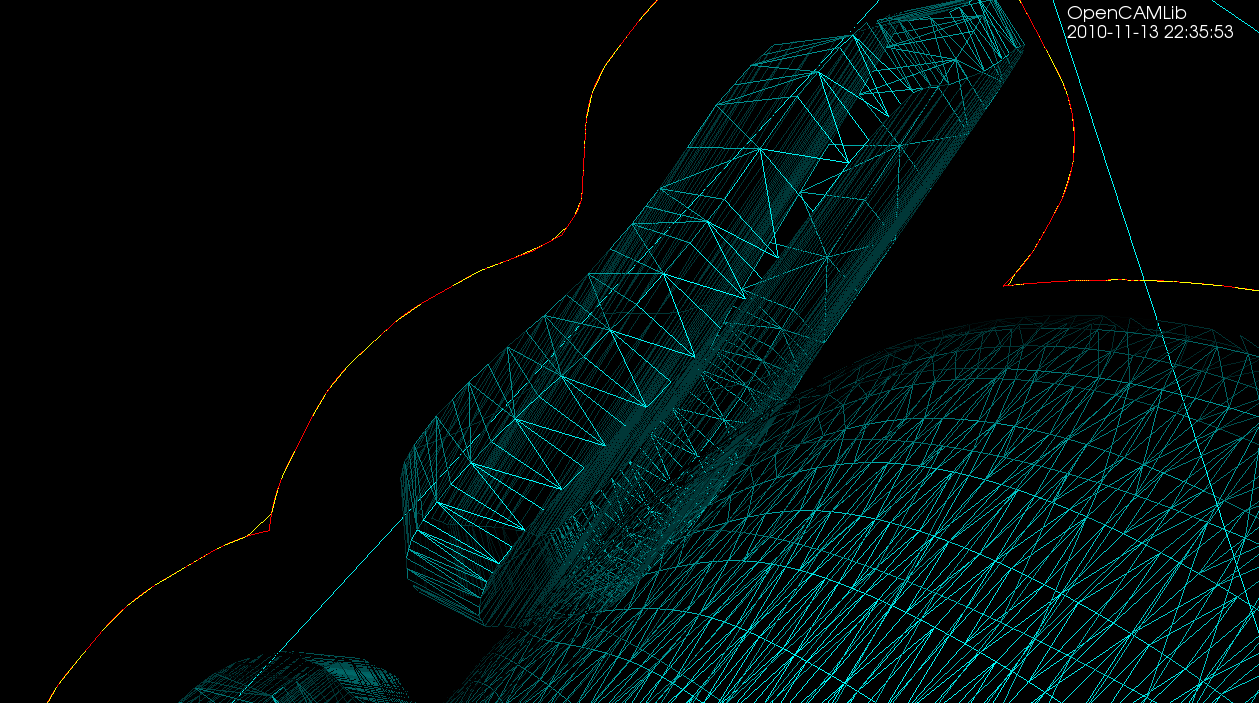
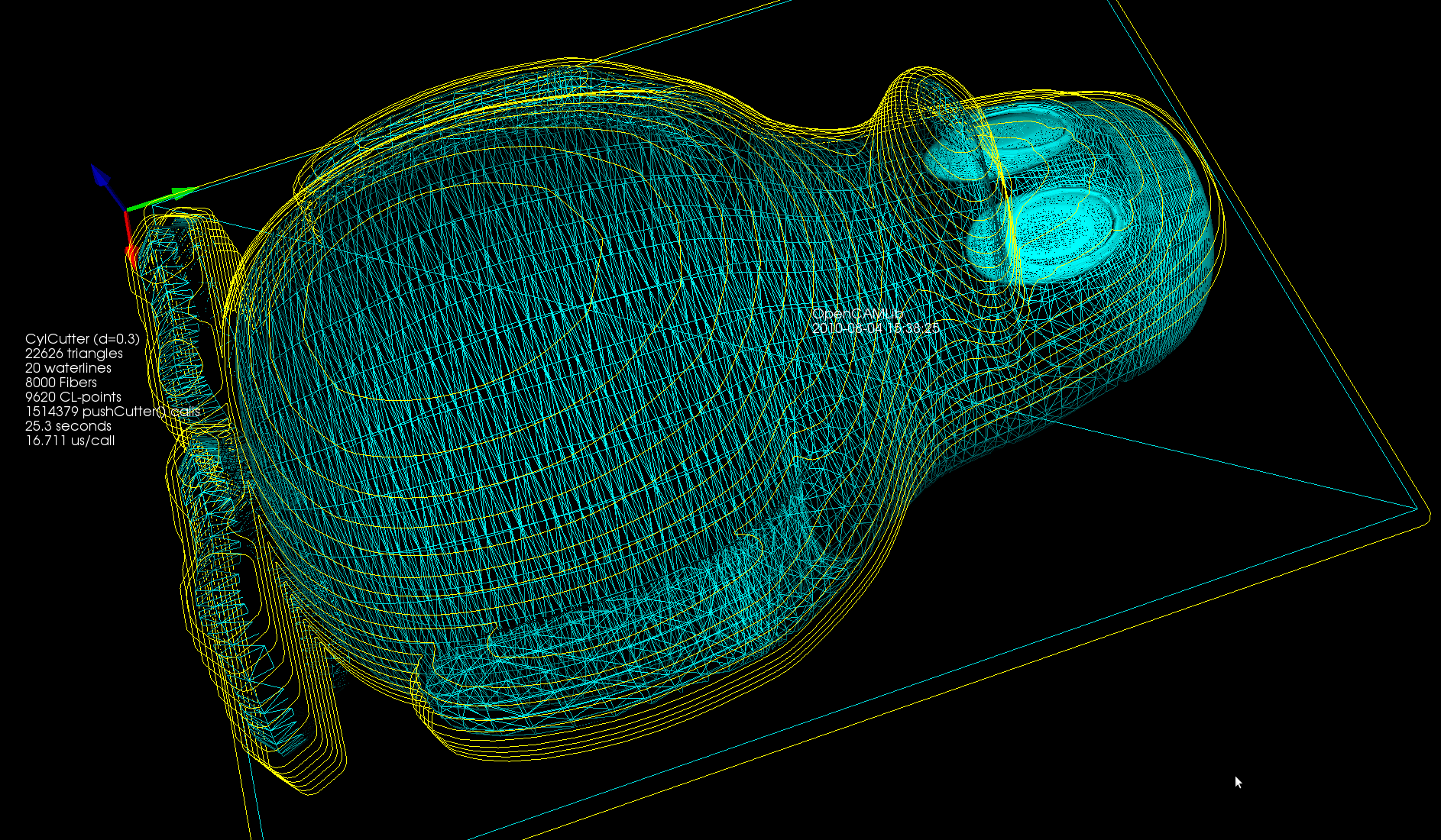
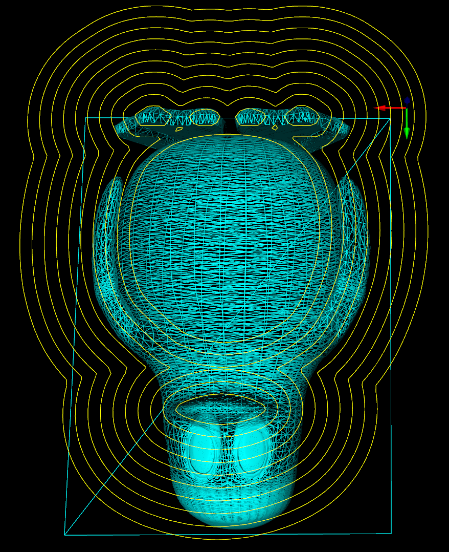
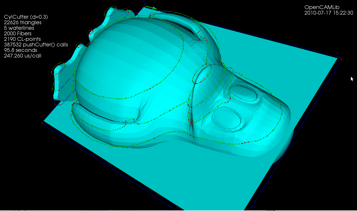
The second test-case is the Tux model where we calculate a single waterline at some z-height. Note how using the chosen ball-cutter at this particular height the waterline splits into two separate loops.

(the yellow line is a plain waterline and the red line is an adaptive Waterline, but that's not important here)

Here is the runtime data. The smaller symbols show results from the one-triangle test-case. The old algorithm(red data points and line) seems to be slower than O(N^2), with a pre-factor of about 2 milliseconds. The time data for the new algorithm (green) fits an O(N^2) line better and has an almost 10-fold faster pre-factor of around 0.25 ms.

The speedup for the Tux model (large symbols) is even greater. With the old algorithm the slope of the data points (pink) looks much worse than N^2 and runtimes quickly reach a minute or more. With the new algorithm (big light green symbols) the runtime stays under 100s even at 200 fibers/mm.

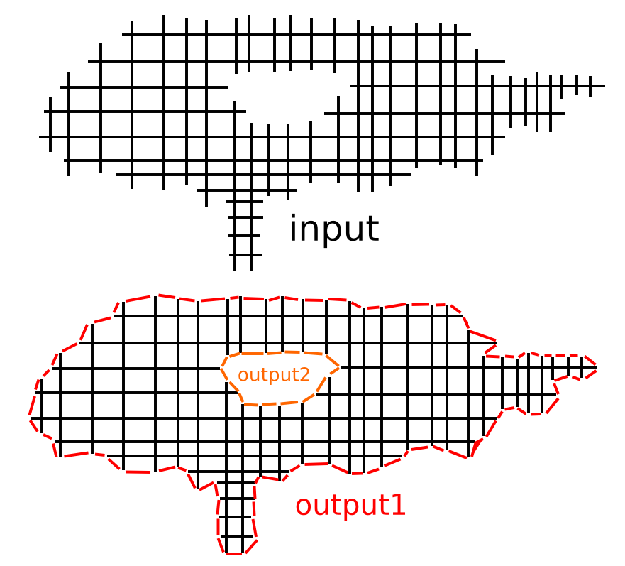
This speedup was achieved by building a weave which is a directed half-edge graph, instead of the old undirected graph. The old algorithm first used connected_components (time complexity O(V + E)) to split the weave into its connected components. For each component a planar embedding was then constructed (time complexity ??), and the toolpath loop extracted with planar_face_traversal (time complexity O(V+E)).

In the new Weave, each edge has a "next" pointer pointing to the next edge of the face. This means we can extract the toolpath loop by following the "next" pointer until we find the next CL-point. Effectively the planar embedding is now contained in the graph datastructure and does not have to be computed separately. This also saves work since we don't have to traverse faces which do not produce toolpaths. This new solution to the weave point-order problemdeserves its own post in the near future - stay tuned...

Better adaptive waterline

Previously the flat() predicate looked only at the number of intervals contained in a fiber when deciding where to insert new fibers in the adaptive waterline algorithm. Here I've borrowed the same flat() function used in adaptive drop-cutter which computes the angle between subsequent line-segments(yellow), and inserts a new fiber(cyan) if the angle exceeds some pre-set threshold.

This works on the larger Tux model also. However, there's no free lunch: the uniformly sampled waterline (yellow) runs in about 2 s (using OpenMP on a dual-core machine), while the adaptively sampled waterline takes around 30s to compute (no OpenMP).

The difference between the adaptive (red) and the uniformly sampled (yellow) waterlines is really only visible when zooming in on sharp corners or other details. Compare this to adaptive drop-cutter.

Waterline problem

I was trying to work on a new adaptive waterline feature, but ended up uncovering an old existing problem/bug with waterline. I think it has to be a problem in either building the weave from the fibers, or constructing the planar embedding of the weave.

The yellow waterline should obviously be a smooth loop around the outside of the weave (red/green fibers) and not a zigzag journey back and forth... 🙁

Update: this is better now:

Update2: here's a figure where new fibers (red and green) are inserted adaptively where the shape of the waterline changes most. There's something wrong with building the planar embedding for this weave, so no yellow adaptive waterline path yet...

Update3: some progress at last (fixed a bug in adaptive drop-cutter at the same time):

The weave point-order problem

When creating waterlines or 2D offsets using a "sampling" or "CL-point based" approach the result is a grid or weave such as that shown in black above. The black lines can in principle be unevenly spaced, and don't necessarily have to be aligned with the X/Y-axis. The desired output of the operation is shown in red/orage, i.e. a loop around/inside this weave/grid, which connects all the "loose ends" of the graph.

My first approach was to start at any CL-vertex and do a breadth_first_search from there to find the closest neighboring vertices. If there are many candidates equally close you then need to decide where to jump forward, and do the next breadth_first_search. This is not very efficient, since breadth_first_search runs a lot of times (you could stop the search at a depth or 5-6 to make it faster).

The other idea I had was some kind of 'surface tension', or edge removal/relaxation where you would start at an arbitrary point deep inside the black portion of the graph and work your way to the outside as far as possible to find the output. I haven't implemented this so I'm not sure if it will work.

What's the best/fastest way of finding the output? Comments ?!

Update: I am now solving this by first creating a planar embedding of the graph and then running planar_face_traversal with a visitor that records in which order the CL-points were visited. The initial results look good:

Faster waterlines with OpenMP

This example has three times more fibers, and thus also CL-points, than the original one, but it still runs in a reasonable time of ~15s because (1) I hard-coded the matrix-determinant expressions everywhere instead of relying on a slow general purpose function and (2) the batch-processing of the fibers now uses OpenMP in order to put all those multi-cores to work.

(red=vertex contacts, green=facet contacts, blue=edge contacts)

My initial point-ordering scheme based on a complete breadth-first-search at each CL-point is a bit naive and slow (that's not included in the 15s time), so that still needs more work.

Waterline toolpaths, part 3

I've written a function that looks at the weave and produces a boost adjacency-list graph of it. The graph can then be split up into separate disconnected components using connected_components. To illustrate this, the second highest waterline in the picture below has six disconnected components: around the beak, belly, and toes(4). When we know we are dealing with one connected component we pick a starting point at random. I'm then using breadth_first_search from this starting point to find the distance, along the graph, from this starting CL-point to all other CL-points. We choose the point with the minimum distance (along the graph) as the next point. Sometimes many points have the same distance from the source vertex and another way of choosing between them is required (I'm now picking the one which is closest in 2D distance to the source, but this may not be correct). We then mark the newly found CL-point "done", and proceed with another breadth_first_search with this vertex as the source. That means that the graph-search runs N times if we have N CL-points, which is not very efficient...

So, compared to previously, we now have for each waterline a list-of-lists where each sub-list is a loop, or an ordered list of CL-points. The yellow lines connect adjacent CL-points.

There's still a donut-case, where one connected component of the weave produces more than one loop, which the code doesn't handle correctly.

Waterline toolpaths, part 2

After the proof-of-principle waterline experiments two days ago I've modified the KD-tree search so that triangles overlapping with the cutter can be searched for in the XZ and YZ planes (in addition to the XY-plane, which was needed for drop-cutter). This dramatically reduces the number of triangles which go through the pushCutter function and makes it possible to run some tests on small to medium STL files.

Currently all the CL-points come out of the algorithm in an undefined almost random order. I'm just plotting them all and they are closely spaced, so it looks like a path, but the algorithm has no idea in which order the CL-points should be visited. Before these waterlines are of any use a second algorithm is required which inspects the weave and (a) comes up with the number of "loops" or "rings" (what should we name these?) at each waterline and (b) sorts the CL-points in each loop into the right order. The upstream user of these waterline loops can then decide in which order to visit the waterlines at each z-height, and within one waterline in which order to visit the loops. Any CL-point in a loop is as good as any other, so the upstream user can also choose where to start/stop the toolpath around the loop.

My idea for this is to turn the weave in to a graph and use the Boost Graph Library which has a function for returning the number of connected components (part (a) above), and then perhaps the All-pairs shortest path algorithm to find adjacent CL-points (part (b) above). Any other ideas?

Here's the obligatory Tux example, where it took 96 seconds to generate five waterlines.