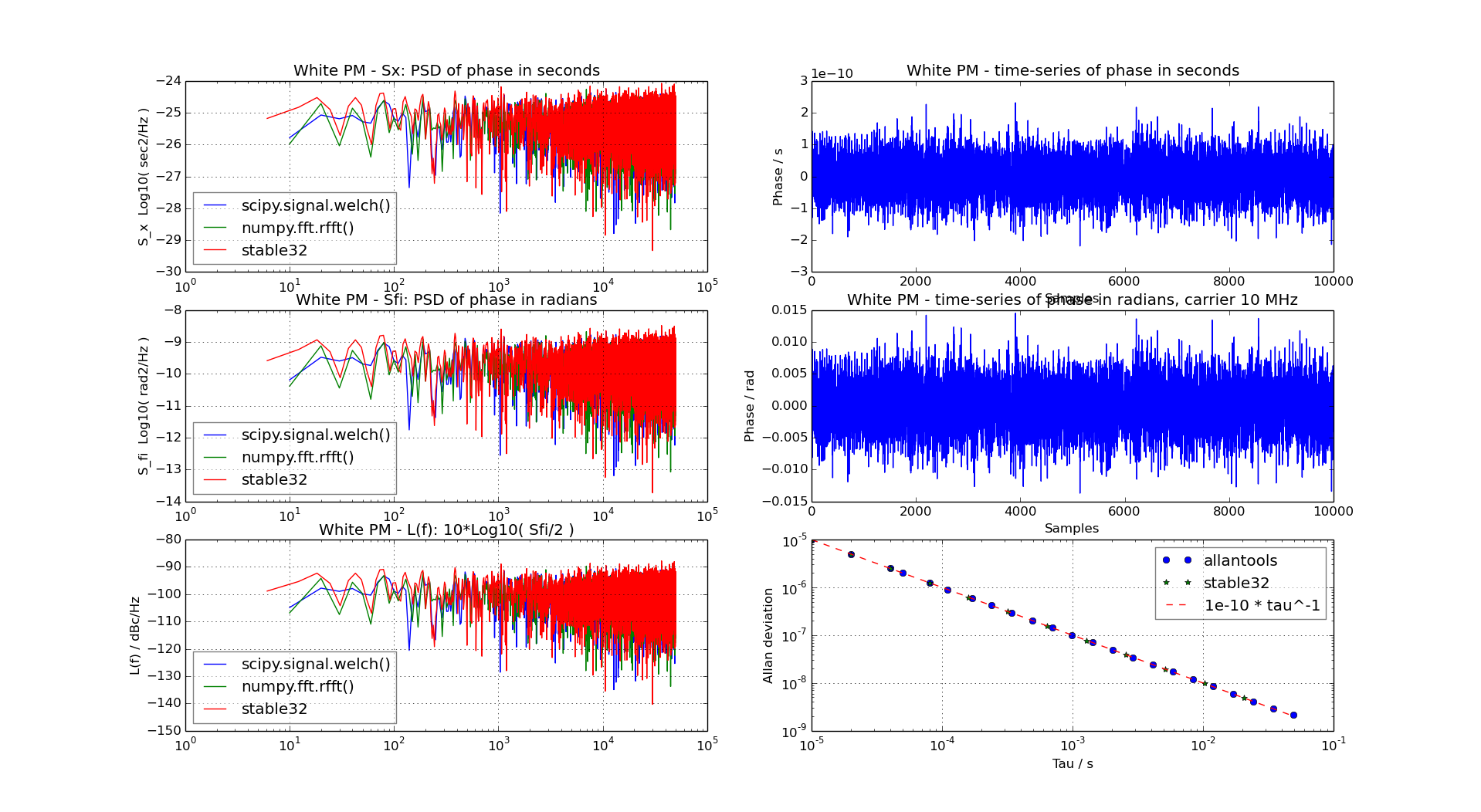
I've looked at calculating phase-noise spectra with python - to be included in allantools. Here are some first results.
I've looked at calculating phase-noise spectra with python - to be included in allantools. Here are some first results.
On github: https://github.com/aewallin/digiclock
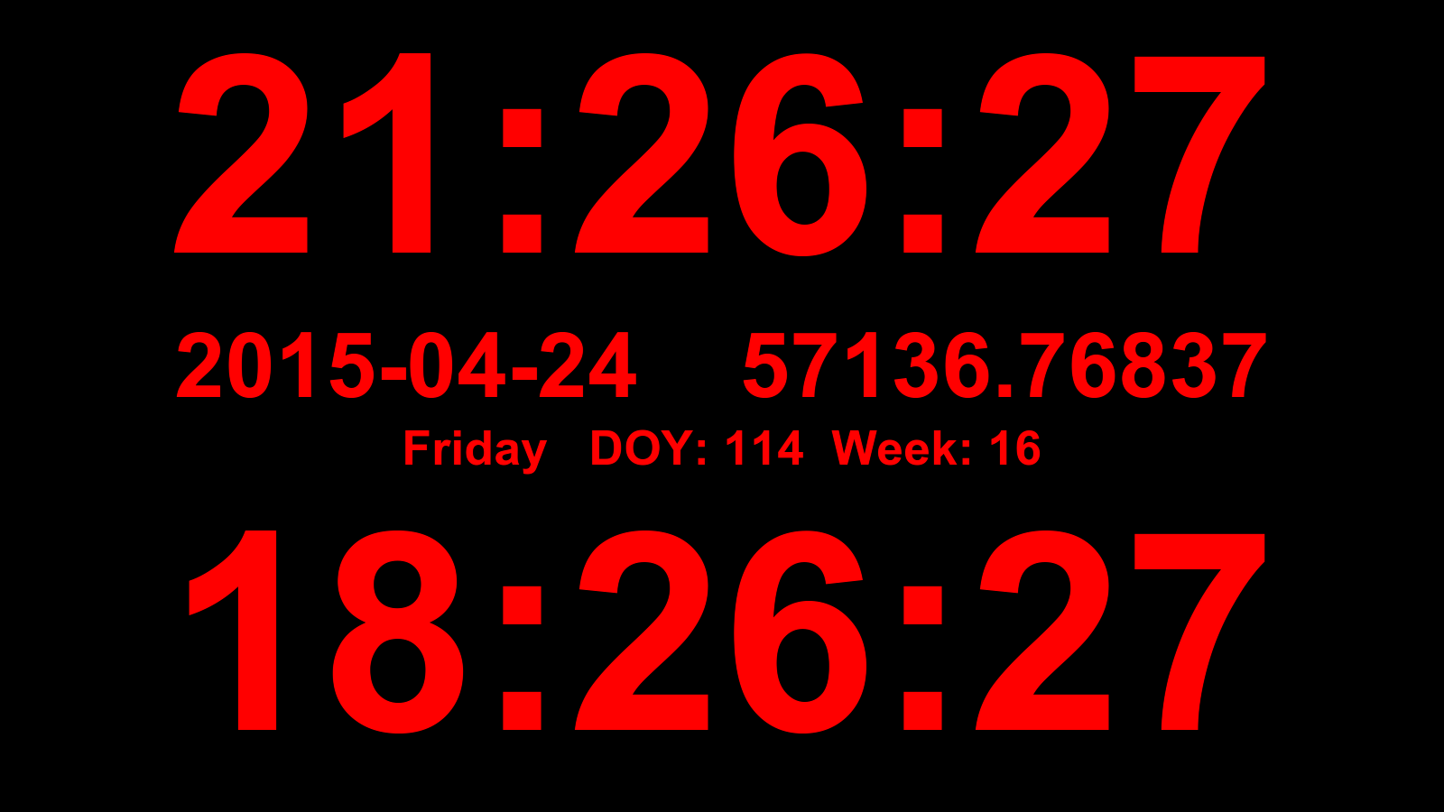
A simple clock display with local time, UTC, date (iso8601 format of course!), MJD, day-of-year, and week number. Useful as a permanent info-display in the lab - just make sure your machines are synced with NTP.
1 2 3 4 5 6 7 8 9 10 11 12 13 14 15 16 17 18 19 20 21 22 23 24 25 26 27 28 29 30 31 32 33 34 35 36 37 38 39 40 41 42 43 44 45 46 47 48 49 50 51 52 53 | # use Tkinter to show a digital clock # tested with Python24 vegaseat 10sep2006 # https://www.daniweb.com/software-development/python/code/216785/tkinter-digital-clock-python # http://en.sharejs.com/python/19617 # AW2015-04-24 # added: UTC, localtime, date, MJD, DOY, week from Tkinter import * import time import jdutil # https://gist.github.com/jiffyclub/1294443 root = Tk() root.attributes("-fullscreen", True) # this should make Esc exit fullscrreen, but doesn't seem to work.. #root.bind('',root.attributes("-fullscreen", False)) root.configure(background='black') #root.geometry("1280x1024") # set explicitly window size time1 = '' clock_lt = Label(root, font=('arial', 230, 'bold'), fg='red',bg='black') clock_lt.pack() date_iso = Label(root, font=('arial', 75, 'bold'), fg='red',bg='black') date_iso.pack() date_etc = Label(root, font=('arial', 40, 'bold'), fg='red',bg='black') date_etc.pack() clock_utc = Label(root, font=('arial', 230, 'bold'),fg='red', bg='black') clock_utc.pack() def tick(): global time1 time2 = time.strftime('%H:%M:%S') # local time_utc = time.strftime('%H:%M:%S', time.gmtime()) # utc # MJD date_iso_txt = time.strftime('%Y-%m-%d') + " %.5f" % jdutil.mjd_now() # day, DOY, week date_etc_txt = "%s DOY: %s Week: %s" % (time.strftime('%A'), time.strftime('%j'), time.strftime('%W')) if time2 != time1: # if time string has changed, update it time1 = time2 clock_lt.config(text=time2) clock_utc.config(text=time_utc) date_iso.config(text=date_iso_txt) date_etc.config(text=date_etc_txt) # calls itself every 200 milliseconds # to update the time display as needed # could use >200 ms, but display gets jerky clock_lt.after(20, tick) tick() root.mainloop() |
This uses two small additions to jdutil:
1 2 3 4 5 6 7 | def mjd_now(): t = dt.datetime.utcnow() return dt_to_mjd(t) def dt_to_mjd(dt): jd = datetime_to_jd(dt) return jd_to_mjd(jd) |
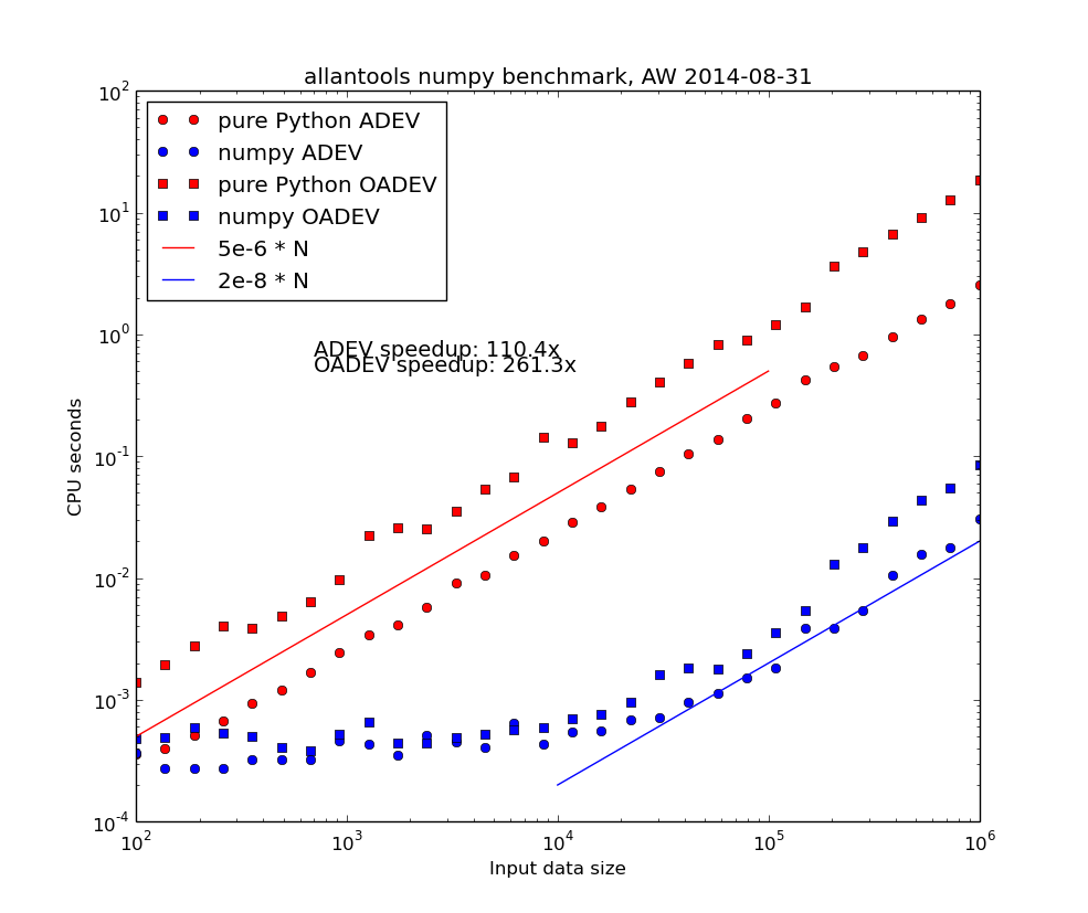
Update: these slopes are both linear, or O(n), where n is the input data size.
However for the worst performing algorithm, MTIE, an O(n*log(n)) algorithm that uses a binary tree to store intermediate results is possible. This algorithm restricts the tau-values to 2**k (with k integer) times the data interval.
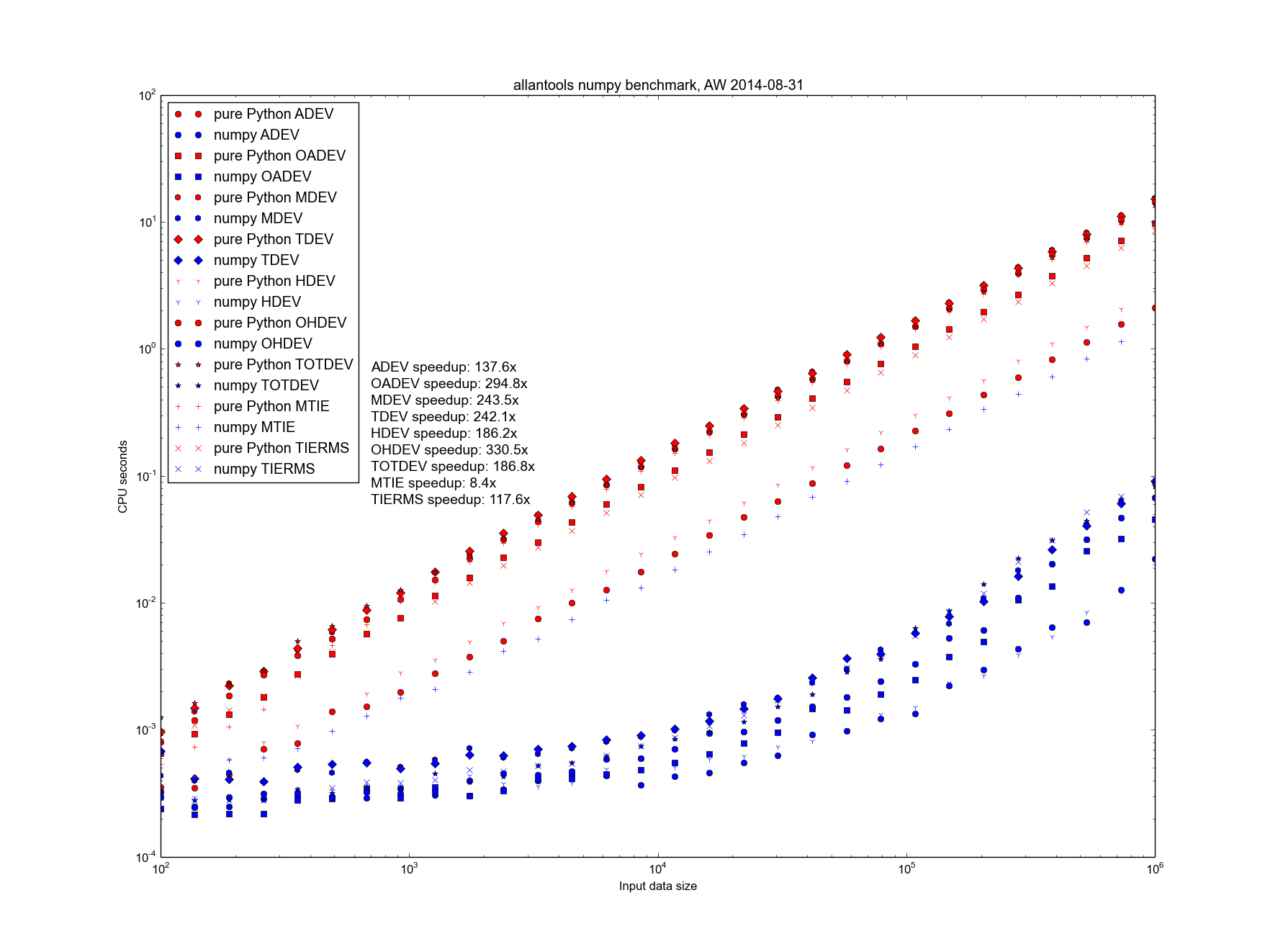
Danny Price has made a fantastic contribution to allantools by taking my previous pure python code (hacked together in January 2014, shown in red) and numpyifying it all (shown in blue)!
For large datasets the speedups are 100-fold or more in most cases!
The speedups are calculated only for datasets larger than 1e5, since python's time.time() doesn't seem suitable for measuring 1 ms or shorter running times.
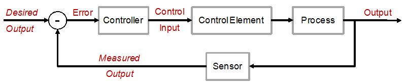
The world is full of PID-loops, thermostats, and PLLs. These are all feedback loops where we control a certain output variable through an input variable, with a more or less known physical process (sometimes called "plant") between input and output. The input or "set-point" is the desired output where we'd like the feedback system to keep our output variable.
Let's say we want to change the set-point. Now what's a reasonable way to do that? If our controller can act infinitely fast we could just jump to the new set-point and hope for the best. In real life the controller, plant, and feedback sensor all have limited bandwidth, and it's unreasonable to ask any feedback system to respond to a sudden change in set-point. We need a Trajectory - a smooth (more or less) time-series of set-point values that will take us from the current set-point to the new desired value.
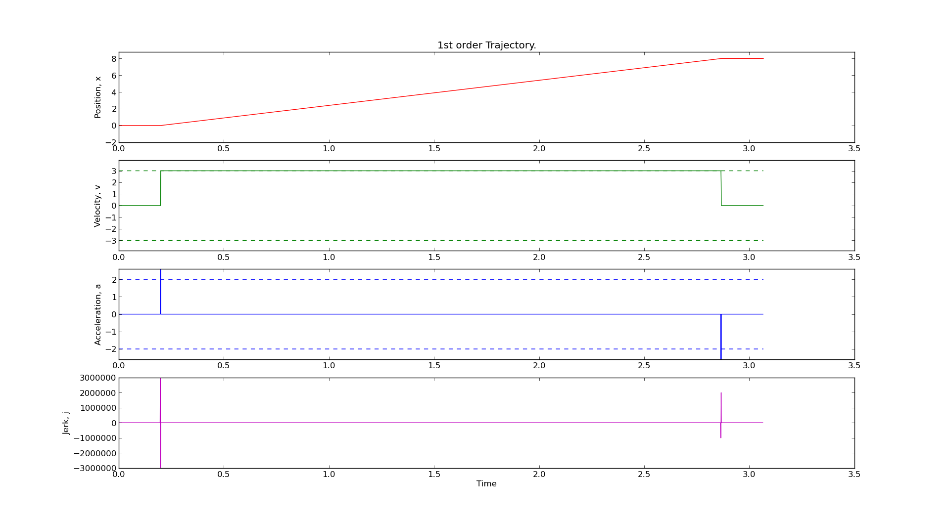
Here are two simple trajectory planners. The first is called 1st order continuous, since the plot of position is continuous. But note that the velocity plot has sudden jumps, and the acceleration & jerk plots have sharp spikes. In a feedback system where acceleration or jerk corresponds to a physical variable with finite bandwidth this will not work well.
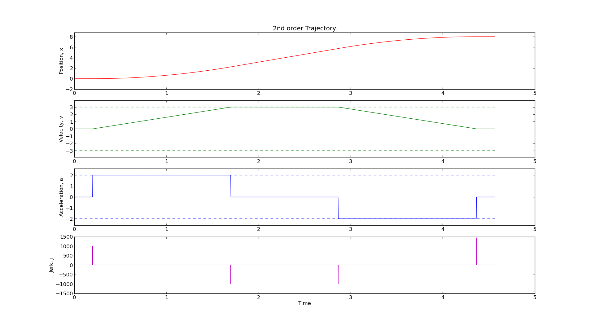
We get a smoother trajectory if we also limit the maximum allowable acceleration. This is a 2nd order trajectory since both position and velocity are continuous. The acceleration still has jumps, and the jerk plot shows (smaller) spikes as before.
Here is the python code that generates these plots:
1 2 3 4 5 6 7 8 9 10 11 12 13 14 15 16 17 18 19 20 21 22 23 24 25 26 27 28 29 30 31 32 33 34 35 36 37 38 39 40 41 42 43 44 45 46 47 48 49 50 51 52 53 54 55 56 57 58 59 60 61 62 63 64 65 66 67 68 69 70 71 72 73 74 75 76 77 78 79 80 81 82 83 84 85 86 87 88 89 90 91 92 93 94 95 96 97 98 99 100 101 102 103 104 105 106 107 108 109 110 111 112 113 114 115 116 117 118 119 120 121 122 123 124 125 126 127 128 129 130 131 132 133 134 135 136 137 138 139 140 141 142 143 144 145 146 147 148 149 150 151 152 153 154 155 156 157 158 159 160 161 162 163 164 165 166 167 168 169 170 171 172 173 174 175 176 177 178 179 180 181 182 183 184 185 186 187 188 189 190 191 192 193 194 195 196 | # AW 2014-03-17 # GPLv2+ license import math import matplotlib.pyplot as plt import numpy # first order trajectory. bounded velocity. class Trajectory1: def __init__(self, ts = 1.0, vmax = 1.2345): self.ts = ts # sampling time self.vmax = vmax # max velocity self.x = float(0) # position self.target = 0 self.v = 0 # velocity self.t = 0 # time self.v_suggest = 0 def setTarget(self, T): self.target = T def setX(self, x): self.x = x def run(self): self.t = self.t + self.ts # advance time sig = numpy.sign( self.target - self.x ) # direction of move if sig > 0: if self.x + self.ts*self.vmax > self.target: # done with move self.x = self.target self.v = 0 return False else: # move with max speed towards target self.v = self.vmax self.x = self.x + self.ts*self.v return True else: # negative direction move if self.x - self.ts*self.vmax < self.target: # done with move self.x = self.target self.v = 0 return False else: # move with max speed towards target self.v = -self.vmax self.x = self.x + self.ts*self.v return True def zeropad(self): self.t = self.t + self.ts def prnt(self): print "%.3f\t%.3f\t%.3f\t%.3f" % (self.t, self.x, self.v ) def __str__(self): return "1st order Trajectory." # second order trajectory. bounded velocity and acceleration. class Trajectory2: def __init__(self, ts = 1.0, vmax = 1.2345 ,amax = 3.4566): self.ts = ts self.vmax = vmax self.amax = amax self.x = float(0) self.target = 0 self.v = 0 self.a = 0 self.t = 0 self.vn = 0 # next velocity def setTarget(self, T): self.target = T def setX(self, x): self.x = x def run(self): self.t = self.t + self.ts sig = numpy.sign( self.target - self.x ) # direction of move tm = 0.5*self.ts + math.sqrt( pow(self.ts,2)/4 - (self.ts*sig*self.v-2*sig*(self.target-self.x)) / self.amax ) if tm >= self.ts: self.vn = sig*self.amax*(tm - self.ts) # constrain velocity if abs(self.vn) > self.vmax: self.vn = sig*self.vmax else: # done (almost!) with move self.a = float(0.0-sig*self.v)/float(self.ts) if not (abs(self.a) <= self.amax): # cannot decelerate directly to zero. this branch required due to rounding-error (?) self.a = numpy.sign(self.a)*self.amax self.vn = self.v + self.a*self.ts self.x = self.x + (self.vn+self.v)*0.5*self.ts self.v = self.vn assert( abs(self.a) <= self.amax ) assert( abs(self.v) <= self.vmax ) return True else: # end of move assert( abs(self.a) <= self.amax ) self.v = self.vn self.x = self.target return False # constrain acceleration self.a = (self.vn-self.v)/self.ts if abs(self.a) > self.amax: self.a = numpy.sign(self.a)*self.amax self.vn = self.v + self.a*self.ts # update position #if sig > 0: self.x = self.x + (self.vn+self.v)*0.5*self.ts self.v = self.vn assert( abs(self.v) <= self.vmax ) #else: # self.x = self.x + (-vn+self.v)*0.5*self.ts # self.v = -vn return True def zeropad(self): self.t = self.t + self.ts def prnt(self): print "%.3f\t%.3f\t%.3f\t%.3f" % (self.t, self.x, self.v, self.a ) def __str__(self): return "2nd order Trajectory." vmax = 3 # max velocity amax = 2 # max acceleration ts = 0.001 # sampling time # uncomment one of these: #traj = Trajectory1( ts, vmax ) traj = Trajectory2( ts, vmax, amax ) traj.setX(0) # current position traj.setTarget(8) # target position # resulting (time, position) trajectory stored here: t=[] x=[] # add zero motion at start and end, just for nicer plots Nzeropad = 200 for n in range(Nzeropad): traj.zeropad() t.append( traj.t ) x.append( traj.x ) # generate the trajectory while traj.run(): t.append( traj.t ) x.append( traj.x ) t.append( traj.t ) x.append( traj.x ) for n in range(Nzeropad): traj.zeropad() t.append( traj.t ) x.append( traj.x ) # plot position, velocity, acceleration, jerk plt.figure() plt.subplot(4,1,1) plt.title( traj ) plt.plot( t , x , 'r') plt.ylabel('Position, x') plt.ylim((-2,1.1*traj.target)) plt.subplot(4,1,2) plt.plot( t[:-1] , [d/ts for d in numpy.diff(x)] , 'g') plt.plot( t , len(t)*[vmax] , 'g--') plt.plot( t , len(t)*[-vmax] , 'g--') plt.ylabel('Velocity, v') plt.ylim((-1.3*vmax,1.3*vmax)) plt.subplot(4,1,3) plt.plot( t[:-2] , [d/pow(ts,2) for d in numpy.diff( numpy.diff(x) ) ] , 'b') plt.plot( t , len(t)*[amax] , 'b--') plt.plot( t , len(t)*[-amax] , 'b--') plt.ylabel('Acceleration, a') plt.ylim((-1.3*amax,1.3*amax)) plt.subplot(4,1,4) plt.plot( t[:-3] , [d/pow(ts,3) for d in numpy.diff( numpy.diff( numpy.diff(x) )) ] , 'm') plt.ylabel('Jerk, j') plt.xlabel('Time') plt.show() |
See also:
I'd like to extend this example, so if anyone has simple math+code for a third-order or fourth-order trajectory planner available, please publish it and comment below!
More zeromq testing. See also PUB/SUB.
This pattern is for a reply&request situation where one machine asks for data from another machine. The pattern enforces an exchange of messages like this:
REQuester always first sends, then receives.
REPlyer always first receives, then sends.
Requester
1 2 3 4 5 6 7 8 9 10 11 12 13 14 15 16 17 18 19 20 21 22 23 24 25 26 27 28 29 30 31 | import zmq import time # request data from this server:port server = "192.168.3.38" port = 6000 context = zmq.Context() socket = context.socket(zmq.REQ) socket.connect ("tcp://%s:%s" % (server,port) ) while True: tstamp = time.time() msg = "%f" % tstamp # just send a timestamp # REQuester: TX first, then RX socket.send(msg) # TX first rep = socket.recv() # RX second done = time.time() oneway = float(rep)-tstamp twoway = done - tstamp print "REQuest ",msg print "REPly %s one-way=%.0f us two-way= %.0f us" % ( rep, 1e6*oneway,1e6*twoway ) time.sleep(1) # typical output: # REQuest 1392043172.864768 # REPly 1392043172.865097 one-way=329 us two-way= 1053 us # REQuest 1392043173.866911 # REPly 1392043173.867331 one-way=420 us two-way= 1179 us # REQuest 1392043174.869177 # REPly 1392043174.869572 one-way=395 us two-way= 1144 us |
The one-way delay here assumes we have machines with synchronized clocks. This might be true to within 1ms or so if both machines are close to the same NTP server.
The two-way delay should be more accurate, since we subtract two time-stamps that both come from the REQuesters system clock. Much better performance can probably be achieved by switching to C or C++.
Replyer:
1 2 3 4 5 6 7 8 9 10 11 12 13 14 15 16 17 18 19 20 21 22 23 24 25 26 | import zmq import time port = 6000 context = zmq.Context() socket = context.socket(zmq.REP) # reply to anyone who asks on this port socket.bind("tcp://*:%s" % port) print "waiting.." while True: # Wait for next request from client message = socket.recv() # RX first print "Received REQuest: ", message tstamp = time.time() sendmsg = "%f" % tstamp # send back a time-stamp print "REPlying: ",sendmsg socket.send(sendmsg) # TX second # typical output: # Received REQuest: 1392043244.206799 # REPlying: 1392043244.207214 # Received REQuest: 1392043245.209014 # REPlying: 1392043245.209458 # Received REQuest: 1392043246.211170 # REPlying: 1392043246.211567 |
I'm playing with zeromq for simple network communication/control. For a nice introduction with diagrams see Nicholas Piel's post "ZeroMQ an introduction"
Here is the PUBlish/SUBscribe patter, which usually consist of one Publisher and one or many Subscribers.
Publisher:
1 2 3 4 5 6 7 8 9 10 11 12 13 14 15 16 17 18 19 20 21 | import zmq from random import choice import time context = zmq.Context() socket = context.socket(zmq.PUB) socket.bind("tcp://*:6000") # publish to anyone listening on port 6000 countries = ['netherlands','brazil','germany','portugal'] events = ['yellow card', 'red card', 'goal', 'corner', 'foul'] while True: msg = choice( countries ) +" "+ choice( events ) print "PUB-> " ,msg socket.send( msg ) # PUBlisher only sends messages time.sleep(2) # output: # PUB-> netherlands yellow card # PUB-> netherlands red card # PUB-> portugal corner |
And here is the Subscriber:
1 2 3 4 5 6 7 8 9 10 11 12 13 14 15 16 17 18 19 | import zmq context = zmq.Context() socket = context.socket(zmq.SUB) # specific server:port to subscribe to socket.connect("tcp://192.168.3.35:6000") # subscription filter, "" means subscribe to everything socket.setsockopt(zmq.SUBSCRIBE, "") print "waiting.." while True: msg = socket.recv() # SUBscriber only receives messages print "SUB -> %s" % msg # typical output: # waiting.. # SUB -> portugal corner # SUB -> portugal foul # SUB -> portugal foul |
Python code for calculating Allan deviation and related statistics: https://github.com/aewallin/allantools
Sample output:
Cheat-sheet (see http://en.wikipedia.org/wiki/Colors_of_noise).
| Phase PSD | Frequency PSD | ADEV |
| 1/f^4, "Black?" | 1/f^2, Brownian, random walk | sqrt(tau) |
| 1/f^3 ?, "Black?" | 1/f Pink | constant |
| 1/f^2, Brownian, random walk | f^0, White | 1/sqrt(tau) |
| f^0, White | f^2 Violet | 1/tau |
Phase PSD is frequency dependence of the the power-spectral-density of the phase noise.
Frequency PSD is the frequency dependence of the power-spectral-density of the frequency noise.
ADEV is the tau-dependence of the Allan deviation.
These can get confusing! Please comment below if I made an error!
I'm experimenting with compiling programs for the N9.
Go to http://harmattan-dev.nokia.com and get their python script harmattan-sdk-setup.py. Make it executable:
chmod a+x harmattan-sdk-setup.py
Run the script as root:
sudo ./harmattan-sdk-setup.py
Press "0" for admininstall. This will start a lengthy install. On my machine it started with installing python-qt4. Then scratchbox (89Mb download for X86 and another 89Mb download for ARM). Then comes the SDK itself, one 825 Mb download for the X86-SDK and another 806 Mb download for the ARMEL-SDK.
Now I get:
:~/Desktop$ scratchbox

bash: /usr/bin/scratchbox: Permission denied
That's because the scratchbox install creates a new user group sbox, and adds your username to this group. We now need to log out of the machine and log in again so that this group is created and your user is added to the group. Now we can run scratchbox. Now, from another terminal on the host-machine, start Xephyr with this:
Xephyr :2 -host-cursor -screen 854x480 -dpi 96 -ac +extension Composite &
From the scratchbox terminal we can now start meego:
meego-sb-session start
This gives a little bit of error-messages, but nothing major I guess. And we have a working "phone":

If we start Xephyr in portrait mode instead with 480x854x16 it looks a bit better: (should also work by passing '-landscape' flag to meego-sb-session)

The screen where all the open applications are shown looks a bit strange:

This environment should allow coding and compiling in the correct environment on X86, and then cross-compiling on the ARMEL-target and packaging into debs for sending to the device. But on IRC I am told there's an alternative QtSDK toolchain that does the same thing - maybe in a simpler way. To be continued...
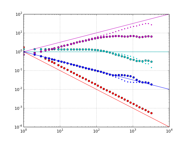
With finite precision numbers, if you take a small number eps, there comes a point when x == x + eps. Here's some code that figures out when that happens:
double epsD(double x) { double r; r = 1000.0; while ( x < (x + r) ) r = r / 2.0; return ( 2.0 * r ); } |
With x around one the resolution limit is roughly at 1e-16 for doubles, and 1e-7 for floats. The top data points show how the relative accuracy stays constant, so at x=1e7 the resolution is only about eps=1 for floats.

Thinking about CAD/CAM related stuff, if you have a fancy top of the line CNC-machine with the longest axis x=1000mm and a theoretical accuracy of one micron, or 0.001mm, then we're at the point where we really should use doubles (which are slower, but how much slower?).
python source for plotting the figure: epsplot.py.tar
It looks like there is no efficient way of updating (adding and removing) triangles in a polydata-surface in VTK, so for the cutting-simulation I am looking at other visualization options. Despite all the tutorials and documentation out there on the interwebs it always takes about two hours to get these "Hello World" examples running...

Download a zip-file with the source and cmake file: (This compiles and runs on Ubuntu 10.04LTS) qtopengl