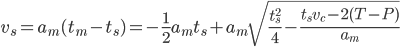
The world is full of PID-loops, thermostats, and PLLs. These are all feedback loops where we control a certain output variable through an input variable, with a more or less known physical process (sometimes called "plant") between input and output. The input or "set-point" is the desired output where we'd like the feedback system to keep our output variable.
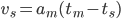
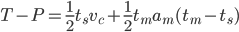
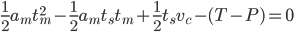
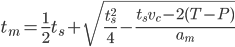
Let's say we want to change the set-point. Now what's a reasonable way to do that? If our controller can act infinitely fast we could just jump to the new set-point and hope for the best. In real life the controller, plant, and feedback sensor all have limited bandwidth, and it's unreasonable to ask any feedback system to respond to a sudden change in set-point. We need a Trajectory - a smooth (more or less) time-series of set-point values that will take us from the current set-point to the new desired value.
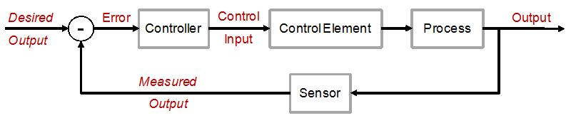
Here are two simple trajectory planners. The first is called 1st order continuous, since the plot of position is continuous. But note that the velocity plot has sudden jumps, and the acceleration & jerk plots have sharp spikes. In a feedback system where acceleration or jerk corresponds to a physical variable with finite bandwidth this will not work well.
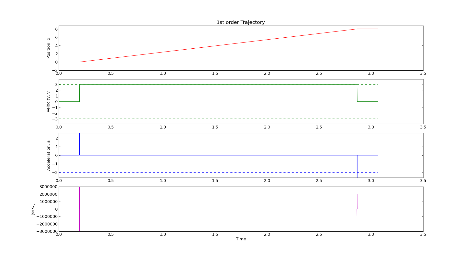
We get a smoother trajectory if we also limit the maximum allowable acceleration. This is a 2nd order trajectory since both position and velocity are continuous. The acceleration still has jumps, and the jerk plot shows (smaller) spikes as before.
Here is the python code that generates these plots:
1 2 3 4 5 6 7 8 9 10 11 12 13 14 15 16 17 18 19 20 21 22 23 24 25 26 27 28 29 30 31 32 33 34 35 36 37 38 39 40 41 42 43 44 45 46 47 48 49 50 51 52 53 54 55 56 57 58 59 60 61 62 63 64 65 66 67 68 69 70 71 72 73 74 75 76 77 78 79 80 81 82 83 84 85 86 87 88 89 90 91 92 93 94 95 96 97 98 99 100 101 102 103 104 105 106 107 108 109 110 111 112 113 114 115 116 117 118 119 120 121 122 123 124 125 126 127 128 129 130 131 132 133 134 135 136 137 138 139 140 141 142 143 144 145 146 147 148 149 150 151 152 153 154 155 156 157 158 159 160 161 162 163 164 165 166 167 168 169 170 171 172 173 174 175 176 177 178 179 180 181 182 183 184 185 186 187 188 189 190 191 192 193 194 195 196 | # AW 2014-03-17 # GPLv2+ license import math import matplotlib.pyplot as plt import numpy # first order trajectory. bounded velocity. class Trajectory1: def __init__(self, ts = 1.0, vmax = 1.2345): self.ts = ts # sampling time self.vmax = vmax # max velocity self.x = float(0) # position self.target = 0 self.v = 0 # velocity self.t = 0 # time self.v_suggest = 0 def setTarget(self, T): self.target = T def setX(self, x): self.x = x def run(self): self.t = self.t + self.ts # advance time sig = numpy.sign( self.target - self.x ) # direction of move if sig > 0: if self.x + self.ts*self.vmax > self.target: # done with move self.x = self.target self.v = 0 return False else: # move with max speed towards target self.v = self.vmax self.x = self.x + self.ts*self.v return True else: # negative direction move if self.x - self.ts*self.vmax < self.target: # done with move self.x = self.target self.v = 0 return False else: # move with max speed towards target self.v = -self.vmax self.x = self.x + self.ts*self.v return True def zeropad(self): self.t = self.t + self.ts def prnt(self): print "%.3f\t%.3f\t%.3f\t%.3f" % (self.t, self.x, self.v ) def __str__(self): return "1st order Trajectory." # second order trajectory. bounded velocity and acceleration. class Trajectory2: def __init__(self, ts = 1.0, vmax = 1.2345 ,amax = 3.4566): self.ts = ts self.vmax = vmax self.amax = amax self.x = float(0) self.target = 0 self.v = 0 self.a = 0 self.t = 0 self.vn = 0 # next velocity def setTarget(self, T): self.target = T def setX(self, x): self.x = x def run(self): self.t = self.t + self.ts sig = numpy.sign( self.target - self.x ) # direction of move tm = 0.5*self.ts + math.sqrt( pow(self.ts,2)/4 - (self.ts*sig*self.v-2*sig*(self.target-self.x)) / self.amax ) if tm >= self.ts: self.vn = sig*self.amax*(tm - self.ts) # constrain velocity if abs(self.vn) > self.vmax: self.vn = sig*self.vmax else: # done (almost!) with move self.a = float(0.0-sig*self.v)/float(self.ts) if not (abs(self.a) <= self.amax): # cannot decelerate directly to zero. this branch required due to rounding-error (?) self.a = numpy.sign(self.a)*self.amax self.vn = self.v + self.a*self.ts self.x = self.x + (self.vn+self.v)*0.5*self.ts self.v = self.vn assert( abs(self.a) <= self.amax ) assert( abs(self.v) <= self.vmax ) return True else: # end of move assert( abs(self.a) <= self.amax ) self.v = self.vn self.x = self.target return False # constrain acceleration self.a = (self.vn-self.v)/self.ts if abs(self.a) > self.amax: self.a = numpy.sign(self.a)*self.amax self.vn = self.v + self.a*self.ts # update position #if sig > 0: self.x = self.x + (self.vn+self.v)*0.5*self.ts self.v = self.vn assert( abs(self.v) <= self.vmax ) #else: # self.x = self.x + (-vn+self.v)*0.5*self.ts # self.v = -vn return True def zeropad(self): self.t = self.t + self.ts def prnt(self): print "%.3f\t%.3f\t%.3f\t%.3f" % (self.t, self.x, self.v, self.a ) def __str__(self): return "2nd order Trajectory." vmax = 3 # max velocity amax = 2 # max acceleration ts = 0.001 # sampling time # uncomment one of these: #traj = Trajectory1( ts, vmax ) traj = Trajectory2( ts, vmax, amax ) traj.setX(0) # current position traj.setTarget(8) # target position # resulting (time, position) trajectory stored here: t=[] x=[] # add zero motion at start and end, just for nicer plots Nzeropad = 200 for n in range(Nzeropad): traj.zeropad() t.append( traj.t ) x.append( traj.x ) # generate the trajectory while traj.run(): t.append( traj.t ) x.append( traj.x ) t.append( traj.t ) x.append( traj.x ) for n in range(Nzeropad): traj.zeropad() t.append( traj.t ) x.append( traj.x ) # plot position, velocity, acceleration, jerk plt.figure() plt.subplot(4,1,1) plt.title( traj ) plt.plot( t , x , 'r') plt.ylabel('Position, x') plt.ylim((-2,1.1*traj.target)) plt.subplot(4,1,2) plt.plot( t[:-1] , [d/ts for d in numpy.diff(x)] , 'g') plt.plot( t , len(t)*[vmax] , 'g--') plt.plot( t , len(t)*[-vmax] , 'g--') plt.ylabel('Velocity, v') plt.ylim((-1.3*vmax,1.3*vmax)) plt.subplot(4,1,3) plt.plot( t[:-2] , [d/pow(ts,2) for d in numpy.diff( numpy.diff(x) ) ] , 'b') plt.plot( t , len(t)*[amax] , 'b--') plt.plot( t , len(t)*[-amax] , 'b--') plt.ylabel('Acceleration, a') plt.ylim((-1.3*amax,1.3*amax)) plt.subplot(4,1,4) plt.plot( t[:-3] , [d/pow(ts,3) for d in numpy.diff( numpy.diff( numpy.diff(x) )) ] , 'm') plt.ylabel('Jerk, j') plt.xlabel('Time') plt.show() |
See also:
- EMC2 tpRunCycle revisited and the correspoinding LinuxCNC wiki page
- Lambrechts 2004 paper, with step by step instructions for generating a 4th order trajectory.
- or a longer report by Lambrecht on the same subject
I'd like to extend this example, so if anyone has simple math+code for a third-order or fourth-order trajectory planner available, please publish it and comment below!