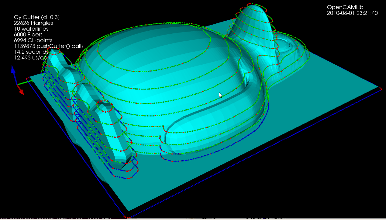
I've written a function that looks at the weave and produces a boost adjacency-list graph of it. The graph can then be split up into separate disconnected components using connected_components. To illustrate this, the second highest waterline in the picture below has six disconnected components: around the beak, belly, and toes(4). When we know we are dealing with one connected component we pick a starting point at random. I'm then using breadth_first_search from this starting point to find the distance, along the graph, from this starting CL-point to all other CL-points. We choose the point with the minimum distance (along the graph) as the next point. Sometimes many points have the same distance from the source vertex and another way of choosing between them is required (I'm now picking the one which is closest in 2D distance to the source, but this may not be correct). We then mark the newly found CL-point "done", and proceed with another breadth_first_search with this vertex as the source. That means that the graph-search runs N times if we have N CL-points, which is not very efficient...
So, compared to previously, we now have for each waterline a list-of-lists where each sub-list is a loop, or an ordered list of CL-points. The yellow lines connect adjacent CL-points.
There's still a donut-case, where one connected component of the weave produces more than one loop, which the code doesn't handle correctly.