pocketing – anderswallin.net

DXF Offset Pocketing loops

Some basic pocketing loops generated on the train today.

Using pycam's revise_directions() function it is possible to clean up the DXF data and classify polygons into pockets and islands.

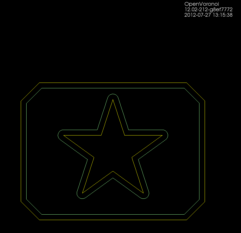
There's a new parameter N_offsets

N_offsets=1 generates just a single offset at a specified offset-distance.
N_offsets=2... generates the specified number of offsets. Possibly with an increment in offset-distance that is not equal to the initial offset-distance. This happens e.g. when we want the final pass of the tool to be one cutter-radius from the input geometry but the material is difficult to machine and we want the "step-over" for interior offset-loops to be less than the cutter-radius.
N_offsets=-1 produces a complete interior pocketing path. Offsets are first generated at the initial offset distance and successive offsets are then generated at increasing offset distance until no offset-output is generated.

Todo: Nesting, Linking, Optimization.

There's no nesting among the loops here. The algorithm will have no clue in what order to machine the offset loops. A naive approach is to machine all loops at the maximum offset distance, then move one loop outwards, etc. But this is clearly not good as the tool would jump between the growing pockets during machining. Nesting information should be straightforward to extract from the voronoi diagram during offset-generation. The nested loops form a tree/graph, which we traverse in some suitable order to machine the entire pocket.

Also, there is no linking of these loops to eachother. For a machining toolpath one wants to link the offsets to each other so that the tool can be kept down in the material when we move from one offset loop to the next. A simple algorithm for linking should be straightforward, but I suspect something more involved is required to prevent overcutting with sufficiently complex input geometry.

When one has nested and linked offset paths, in general there still will remain "pen-up", "rapid traverse", "pen down" transitions. An asymmetric TSP solver could be run on this to minimize the rapid traverse distance (machining time).

More Medial-Axis pocket milling

My first attempt at MA-pocketing only worked when the medial axis of the pocket was a tree (a connected acyclig graph).

I've now extended this to work with pockets consisting of many parts which ha a MA consisting of multiple connected components. There's also simple support for when the MA has cycles, such as seen in "P" and "O" above. With a large cut-width the toolpath looks like this:

Each component of the pocket starts at the red dot with a pink spiral that clears the largest MIC of the pocket. The rest of the pocket is then "scooped out" using green cut-arcs connected with cyan (tool down) or magenta (tool up, at clearance height) rapid moves.

Instead of clearing the interior of letters we can also clear a pocket around the letters. The MA then looks like this:

This video shows quite a lot of "air-cutting". This is because the algorithm only keeps track of the previously cleared area behind the MIC that is currently being cleared. When we come to the end of a cycle in the MA the algorithm does not know that in fact MICs in front of the current MIC have already been cleared.

Medial-Axis pocketing

Update: In the US, where they are silly enough to have software-patents, there's US Patent number: 7831332, "Engagement Milling", Filing date: 29 May 2008, Issue date: 9 Nov 2010. By Inventors: Alan Diehl, Robert B. Patterson of SURFWARE, INC.

Any pocket milling strategy will have as input a step-over distance set at maybe 10 to 90% of the cutter diameter, depending on machine/material/cutter. Zigzag and offset pocketing paths mostly maintain this set step-over, but overload the cutter at sharp corners. Anyone who has tried to cnc-mill a hard material (steel) using a small cnc-mill will know about this. So we want a pocketing path that guarantees a maximum step-over value at all times. Using the medial-axis it is fairly straightforward to come up with a simple pocketing/clearing strategy that achieves this. There are probably many variations on this - the images/video below show only a simple variant I hacked together in 2-3 days.

The medial-axis (MA, blue) of a pocket (yellow) carries with it a clearance-disk radius value. If we place a circle with this radius on the medial-axis, no parts of the pocket boundary will fall within the circle. If we choose a point in the middle of an MA-edge the clearance-disk will touch the polygon at two points. If we choose an MA-vertex of degree three (where three MA-edges meet), the clearance-disk will touch the pocket at three points.

MA-pocketing starts by clearing the largest clearance-disk using a spiral path (pink).

From the maximum clearance-disk we then proceed to clear the rest of the pocket by making cuts along adjacent clearance-disks. We move forward along the MA-graph by an amount that ensures that the step-over width will never be exceeded. The algorithm loops through all clearance-disks and connects the arc-cuts together with bi-tangents, lead-out-arcs, rapids, and lead-in-arcs.

This video shows how it all works (watch in HD!). Here the cutter has 10mm diameter and the step-over is 3mm.

I'll try to make a variant of this for the case where we clear all stock around a central island next. These two variants will be needed for 3D z-terrace roughing.

Towards medial-axis pocketing

Update: some work on connecting MICs together with bi-tangent line-segments, as well as a sequence of lead-out, rapid, lead-in, between successive MIC-slices:

It gets quite confusing with all cutting and non-cutting moves drawn in one image. The path starts with an Archimedean spiral (pink) that clears the initial largest MIC. We then proceed to "scoop" out the rest of the pocket with circular-arc cutting moves (green). At the end of a scoop we do a lead-out-arc (dark blue), followed by a linear rapid (cyan), and a lead-in-arc (light blue) to start the next scoop.

Next I'd like to put together an animation of this. The overall strategy will be much clearer from a movie.

This animation shows MICs, i.e. maximal inscribed circles (green, also called clearance-disks), inside a simple polygon (yellow). The largest MIC is shown in red.

This is work towards a new medial-axis pocketing strategy. The largest MIC (red) is first cleared using a spiral strategy. We then proceed to clear the rest of the pocket in the order that the MICs are drawn in the animation. We don't have to spin the tool around the whole circle. only the parts that need machining, which is the part of the new MIC that doesn't fall inside the previously machined MIC. As mentioned in my previous post this is inspired by Elber et al (2006).

The next step is to calculate how we should proceed from one MIC to the next, and how we do the rapid-traverse to re-position the tool for the next cut.

See also the spiral-toolpath by Held&Spielberger (2009) or their 199-slide presentation. The basics of this spiral-strategy is a straightforward march along the medial-axis. But then a filtering/fitting algorithm, which I don't have at hand right now, is applied to get the smoothed spiral-path.

Voronoi diagram algorithm

Update: now seems to work for at least 10k generators:

and a zoom-in of the same picture:

One way to compute 2D offsets for toolpath generation is via the voronoi diagram. This video shows the first (somehow) working implementation of my code, which is based on papers by Sugihara and Iri. Their 1992 paper is here: http://dx.doi.org/10.1109/5.163412, then a longer 50-page paper from 1994 here: http://dx.doi.org/10.1142/S0218195994000124, and then there's a more general description of the topology-based approach from 1999 here 10.1007/3-540-46632-0_36, and from 2000 here: http://dx.doi.org/10.1007/s004530010002

The algorithm works by incrementally constructing the diagram while adding the point-generators one by one. This initial configuration is used at the beginning:

The diagram will be correct if new generator points are placed inside the orange circle (this way we avoid edges that extend to infinity). Once about 500 randomly chosen points are added the diagram looks like this:

Because of floating-point errors it gets harder to construct the correct diagram when more and more points are added. My code now crashes at slightly more than 500 generators (due to an assert() that fails, not a segfault - yay!). It boils down to calculating the sign of a 4-by-4 determinant, which due to floating-point error goes wrong at some point. That's why the Sugihara-Iri algorithm is based on strictly preserving the correct topology of the diagram, and in fact they show in their papers that their algorithm doesn't crash when a random error is added to the determinant-calculations, and it even works (in some sense) when the determinant calculation is completely replaced by a random number generator. Their 1992 paper constructs the diagram for one million generators using 32-bit float
numbers, while my naive attempt using double here crashes after 535 points... some work to do still then!

CAM toolpaths tend to be based on CAD-geometry in the form of lines, circular arcs, or spline-curves and such. One way forward is to think of a curve as a lot of closely spaced points along the curve. There are also papers which describe how to extend the algorithm for line and arc generators. See the 1996 paper by Imai. There is FORTRAN code for this by Imai over here (I haven't looked at it or tried compiling it...). Held et al. describe voronoi diagram generation for points and lines in 2001: http://dx.doi.org/10.1016/S0925-7721(01)00003-7 and for points, lines, and arcs in 2009 http://dx.doi.org/10.1016/j.cad.2008.08.004. This pic from the Held&Huber 2009 paper shows point, line, and arc generators in bold-black, the associated voronoi-diagram as solid lines, and offsets as grey lines.

Held has more pictures here: http://www.cosy.sbg.ac.at/~held/projects/pocket_off/pocket.html

Note how within one voronoi-region the offset is determined by the associated generator (a line, point, or arc). It's very easy to figure out the offset within one region: points and arcs have circular offsets, while lines have line offsets. The complete offset path is a result of connecting the offset from one region with the next region.