


Histrogams of finishing times scraped from the official website with these scripts: sthlm_scrape
Some more of these over here: https://picasaweb.google.com/106188605401091280402/StockholmMarathonJune22012
Histrogams of finishing times scraped from the official website with these scripts: sthlm_scrape
Some more of these over here: https://picasaweb.google.com/106188605401091280402/StockholmMarathonJune22012
I started working on arc-sites for OpenVoronoi. The first things required are an in_region(p) predicate and an apex_point(p) function. It is best to rapidly try out and visualize things in python/VTK first, before committing to slower coding and design in c++.
in_region(p) returns true if point p is inside the cone-of-influence of the arc site. Here the arc is defined by its start-point p1, end-point p2, center c, and a direction flag cw for indicating cw or ccw direction. This code will only work for arcs smaller than 180 degrees.
def arc_in_region(p1,p2,c,cw,p): if cw: return p.is_right(c,p1) and (not p.is_right(c,p2)) else: return (not p.is_right(c,p1)) and p.is_right(c,p2) |

Here randomly chosen points are shown green if they are in-region and pink if they are not.
apex_point(p) returns the closest point to p on the arc. When p is not in the cone-of-influence either the start- or end-point of the arc is returned. This is useful in OpenVoronoi for calculating the minimum distance from p to any point on the arc-site, since this is given by (p-apex_point(p)).norm().
def closer_endpoint(p1,p2,p): if (p1-p).norm() < (p2-p).norm(): return p1 else: return p2 def projection_point(p1,p2,c1,cw,p): if p==c1: return p1 else: n = (p-c1) n.normalize() return c1 + (p1-c1).norm()*n def apex_point(p1,p2,c1,cw,p): if arc_in_region(p1,p2,c1,cw,p): return projection_point(p1,p2,c1,cw,p) else: return closer_endpoint(p1,p2,p) |

Here a line from a randomly chosen point p to its apex_point(p) has been drawn. Either the start- or end-point of the arc is the closest point to out-of-region points (pink), while a radially projected point on the arc-site is closest to in-region points (green).
The next thing required are working edge-parametrizations for the new type of voronoi-edges that will occur when we have arc-sites (arc/point, arc/line, and arc/arc).
For exploring and visualizing various pocketing or area-clearing milling toolpath strategies I am thinking about reviving the "pixel-mowing" idea from 2007. This would be simply a bitmap with different color for stock remaining and already cleared area. It would be nice to log and/or plot the material removal rate (MRR), or the cutter engagement angle. Perhaps graph it next to the simulation, or create a simulated spindle-soundtrack which would e.g. have a pitch proportional to the inverse of the MRR. It should be possible to demonstrate how the MRR spikes at sharp corners with classical zigzag and offset pocketing strategies. The solution is some kind of HSM-strategy where the MRR is kept below a given limit at all times.
My plan is to play with maximally-inscribed-circles, which are readily available from the medial-axis, like Elber et. al (2006).
Anyway the first step is to render a bitmap in VTK, together with the tool/toolpath, and original pocket geometry:

import vtk import math vol = vtk.vtkImageData() vol.SetDimensions(512,512,1) vol.SetSpacing(1,1,1) vol.SetOrigin(0,0,0) vol.AllocateScalars() vol.SetNumberOfScalarComponents(3) vol.SetScalarTypeToUnsignedChar() scalars = vtk.vtkCharArray() red = [255,0,0] blue= [0,0,255] green= [0,255,0] for n in range(512): for m in range(512): x = 512/2 -n y = 512/2 -m d = math.sqrt(x*x+y*y) if ( d < 100 ): col = red elif (d<200): col = green else: col = blue for c in range(3): scalars.InsertTuple1( n*(512*3) + m*3 +c, col[c] ) vol.GetPointData().SetScalars(scalars) vol.Update() ia = vtk.vtkImageActor() ia.SetInput(vol) ia.InterpolateOff() ren = vtk.vtkRenderer() ren.AddActor(ia) renWin = vtk.vtkRenderWindow() renWin.AddRenderer(ren) iren = vtk.vtkRenderWindowInteractor() iren.SetRenderWindow(renWin) interactorstyle = iren.GetInteractorStyle() interactorstyle.SetCurrentStyleToTrackballCamera() camera = vtk.vtkCamera() camera.SetClippingRange(0.01, 1000) camera.SetFocalPoint(255, 255, 0) camera.SetPosition(0, 0.1, 500) camera.SetViewAngle(50) camera.SetViewUp(1, 1, 0) ren.SetActiveCamera(camera) iren.Initialize() iren.Start() |
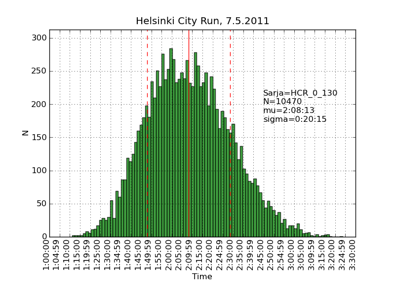
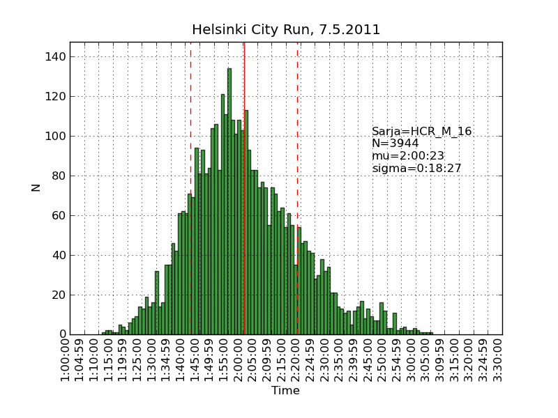
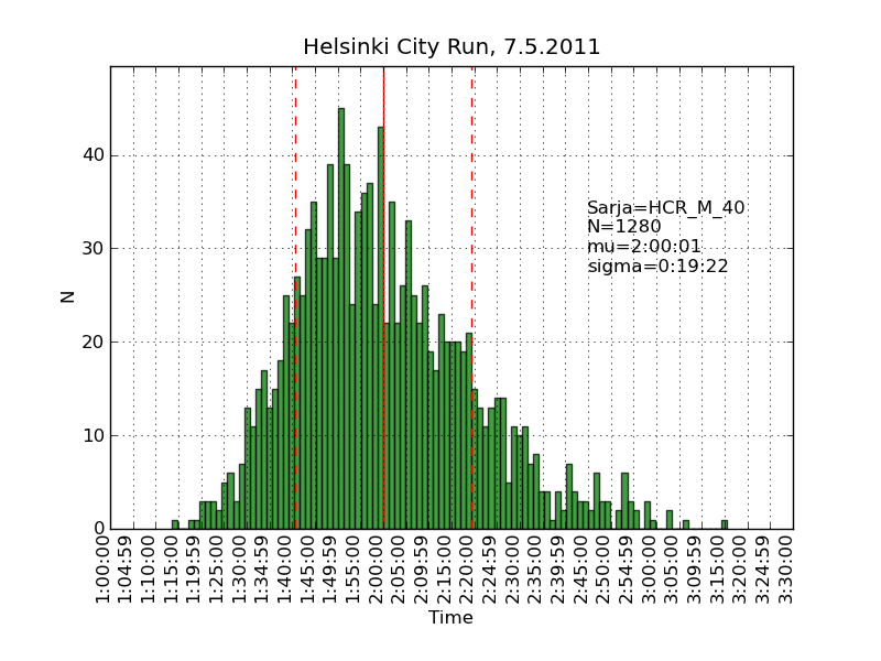
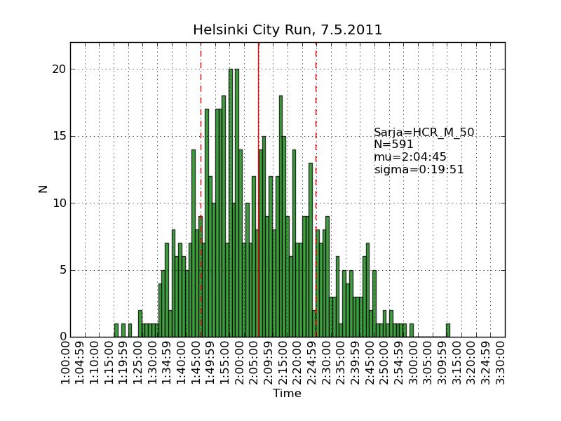
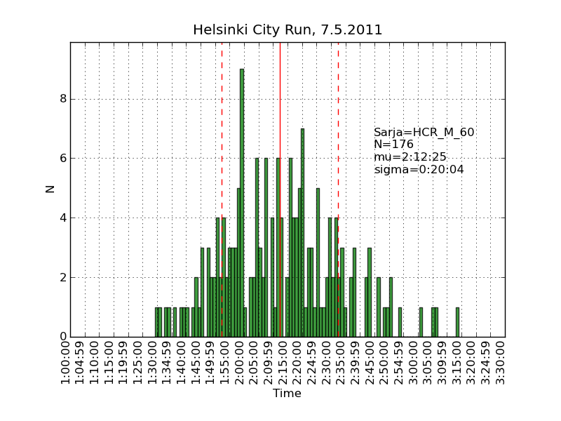
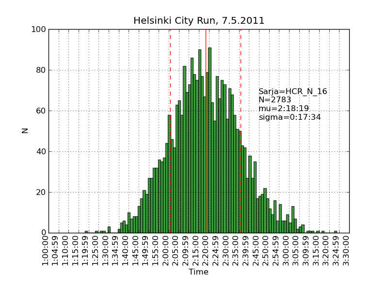
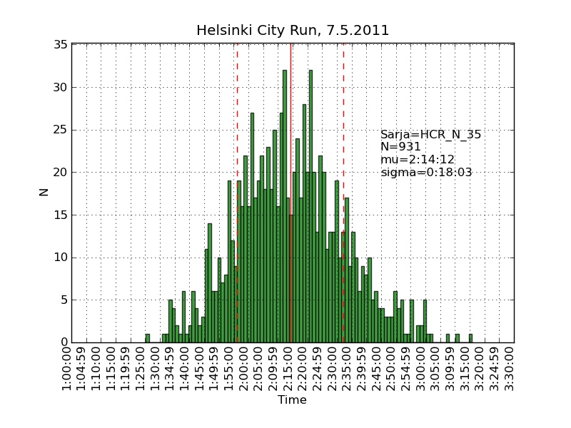
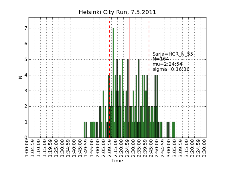
Using the same scraping scripts I wrote after last years marathon, it was fairly easy to scrape the HCR website and produce some histograms.
There are two python scripts, one that crawls the web (urllib) and finds the time-data (BeautifulSoup and re) and writes to a file (cPickle), and another that reads the files and plots (matplotlib) histograms: hcr2011_scrape

Recursion and 'divide-and-conquer' must be two of the greatest ideas ever in computer science.
Threw together some code in python today for building an octree, given a function isInside() which the tree-builder evaluates to see if a node is inside or outside of the object. Nodes completely outside the interesting volume(here a sphere, for simplicity) are rendered grey. Nodes completely inside the object are coloured, green for low tree-depth, and red for high. Where the algorithm can't decide if the node is inside or outside we subdivide (until we reach a decision, or the maximum tree depth).
In the end our sphere-approximation looks something like this:
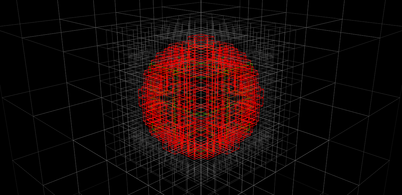
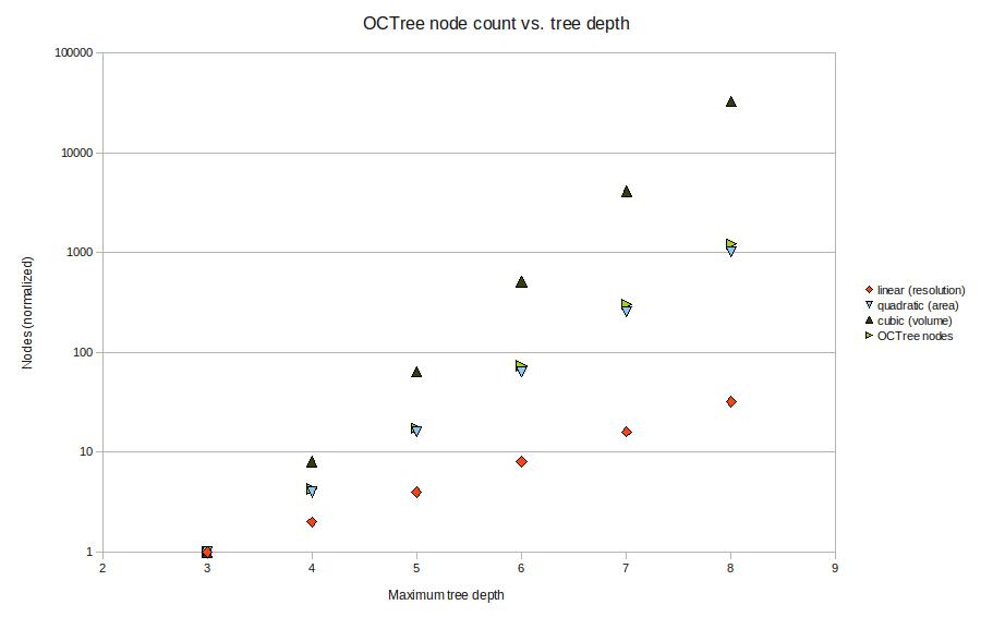
These tests were done with a maximum tree depth of 6 or 7. If we imagine we want a 100 mm long part represented with 0.01 mm precision we will need about depth 14, or a subdivision into 16384 parts. That's impractical to render right now, but seems doable. In terms of memory-use, the octree is much better than a voxel-representation where space is uniformly subdivided into tiny voxels. The graph below shows how the number of nodes grows with tree-depth in the actual octree, versus a voxel-model (i.e. a complete octree). For large tree-depths there are orders-of-magnitude differences, and the octree only uses a number of nodes roughly proportional to the surface area of the part.
Now, the next trick is to implement union (addition) and difference (subtraction) operations for octrees. Then you represent your stock material with one octree, and the tool-swept-volume of your machining operation with another octree -> lo and behold we have a cutting-simulator!

More on the offset-ellipse calculation, which is related to contacting toroidal cutters against edges(lines). An ellipse aligned with the x- and y-axes, with axes a and b can be given in parametric form as (a*cos(theta) , b*sin(theta) ). The ellipse is shown as the dotted oval, in four different colours.
Now the sin() and cos() are a bit expensive the calculate every time you are running this algorithm, so we replace them with parameters (s,t) which are both in [-1,1] and constrain them so s^2 + t^2 = 1, i.e. s = cos(theta) and t=sin(theta). Points on the ellipse are calculated as (a*s, b*t).
Now we need a way of moving around our ellipse to find the one point we are seeking. At point (s,t) on the ellipse, for example the point with the red sphere in the picture, the tangent(shown as a cyan line) to the ellipse will be given by (-a*t, b*s). Instead of worrying about different quadrants in the (s,t) plane, and how the signs of s and t vary, I thought it would be simplest always to take a step in the direction of the tangent. That seems to work quite well, we update s (or t) with a new value according to the tangent, and then t (or s) is calculated from s^2+t^2=1, keeping the sign of t (or s) the same as it was before.
Now for the Newton-Rhapson search we also need a measure of the error, which in this case is the difference in the y-coordinate of the offset-ellipse point (shown as the green small sphere, and obviously calculated as the ellipse-point plus the offset-radius times a normal vector) and where we want that point. Then we just run the algorithm, always stepping either in the positive or negative direction of the tangent along the ellipse, until we reach the required precision (or max number of iterations).
Here's an animation which first shows moving around the ellipse, and then at the end a slowed-down Newton-Rhapson search which in reality converges to better than 8 decimal-places in just seven (7) iterations, but as the animation is slowed down it takes about 60-frames in the movie.
I wonder if all this should be done in Python for the general case too, where the axes of the ellipse are not parallel to the x- and y-axes, before embarking on the c++ version?
Tried to make the code from last time a bit clearer by splitting it into two files:
vtkscreen.py and test2.py
conversion to video again by first converting PNG to JPEG:
mogrify -format jpg -quality 97 *.png
And then encoding JPEGs into a movie:
mencoder mf://*.jpg -mf fps=25:type=jpg -ovc lavc -lavcopts vcodec=mpeg4 -ac copy -o output.avi -ffourcc DX50
I'm trying to learn how to render and animate things using VTK. This is the result of a python-script which outputs a series of PNG-frames. These are then converted to jpegs by this command:
mogrify -format jpg -quality 97 *.png
mencoder mf://*.jpg -mf fps=25:type=jpg -ovc lavc -lavcopts vcodec=mpeg4 -ac copy -o output.avi -ffourcc DX50
This should lead to the revival of my old Drop-Cutter code in the near future. This time it's going to be in C++, with Python bindings, and hopefully use OpenMP. Stay tuned.
As I'm very much an amateur programmer with not too much time to learn new stuff I've decided my CAM-algorithms are going to be written in Python (don't hold your breath, they'll be online when they'll be online...). The benefits of rapid development will more than outweigh the performance issues of Python at this stage.
But then I found Mark Dufour's project shedskin (see also blog here and Mark's MSc thesis here), a Python to C++ compiler! Can you have the best of both worlds? Develop and debug your code interactively with Python and then, when you're happy with it, translate it automagically over to C++ and have it run as fast as native code?
Well, shedskin doesn't support any and all python constructs (yet?), and only a limited number of modules from the standard library are supported. But still I think it's a pretty cool tool. For someone who doesn't look forward to learning C++ from the ground up typing 'shedskin -e myprog.py' followed by 'make' is just a very simple way to create fast python extensions! As a test, I ran shedskin on the pystone benchmark and called both the python and c++ version from my multiprocessing test-code:
Python version
Processes	Pystones	Wall time	pystones/s	Speedup
1		50000		0.7		76171		1.0X
2		100000		0.7		143808		1.9X
3		150000		0.7		208695		2.7X
4		200000		0.8		264410		3.5X
5		250000		1.0		244635		3.2X
6		300000		1.2		259643		3.4X
'shedskinned' C++ version
Processes	Pystones	Wall time		pystones/s	Speedup
1		5000000			2.9		1696625		1.0X
2		10000000		3.1		3234625		1.9X
3		15000000		3.1		4901829		2.9X
4		20000000		3.4		5968676		3.5X
5		25000000		4.4		5714151		3.4X
6		30000000		5.1		5890737		3.5X
A speedup of around 20x.
A simple pystone benchmark using the python multiprocessing package. Seems to scale quite well - guess how many cores my machine has! 🙂
" Simple multiprocessing test.pystones benchmark "
" Anders Wallin 2008Jun15 anders.e.e.wallin (at) gmail.com "
from test import pystone
import processing
import time

STONES_PER_PROCESS= 10*pystone.LOOPS

def f(q):
    t=pystone.pystones(STONES_PER_PROCESS)
    q.put(t,block=True)

if __name__ == '__main__':
    print 'multiprocessing test.pystones() benchmark'
    print 'You have '+str(processing.cpuCount()) + ' CPU(s)'
    print 'Processes\tPystones\tWall time\tpystones/s'

    results = processing.Queue()
    for N in range(1,processing.cpuCount()+3):
        p=[]
        q=processing.Queue()
        results=[]

        for m in range(1,N+1):
            p.append( processing.Process(target=f,args=(q,)) )

        start=time.time()
        for pr in p:
            pr.start()
        for r in p:
            results.append( q.get() )
        stop=time.time()

        cputime = stop-start

        print str(N)+'\t\t'+str(N*STONES_PER_PROCESS) \
              +'\t\t'+ str(cputime)+'\t'+str( N*STONES_PER_PROCESS / cputime )
