Z-map model for 3-axis machining

I've been reading about the z-map model for 3-axis milling. A working simulation environment would be very useful for CAM algorithm development. Coarse errors in the algorithms can be spotted by eye from the simulation, and a comparison of the z-map with the original CAD model can be used to see if the machining really produces the desired part within tolerance.

Jeff Epler hacked together a z-map model with EMC2 a while ago: gdepth. Perhaps some code/ideas can be borrowed from there.

The z-map can also be used for generating the tool paths themselves (similar to bitmap-mowing here, here and here), but that's more advanced and not the immediate goal.

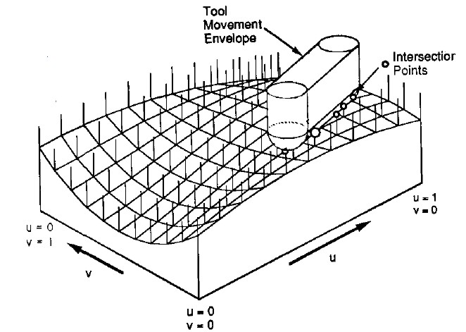
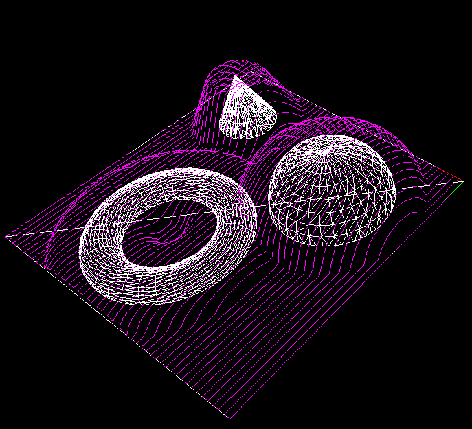
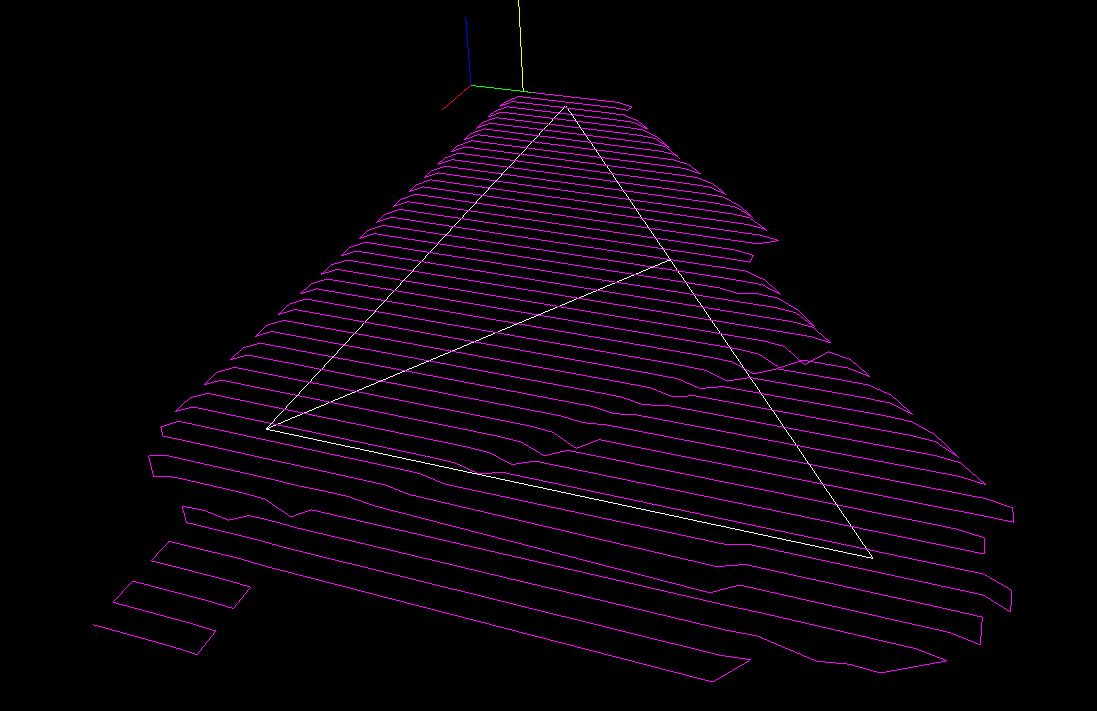
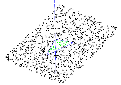
Here's the z-map model, a lot of vectors standing upright in the z-direction, getting cut (or mowed down) by the moving tool. For graphics you could fill each space between four z-vectors with two triangles and display an STL surface. Obviously this works only for 3-axis machining where the tool is oriented along the z-axis, and the tool must also not produce undercuts (e.g. T-slot milling).

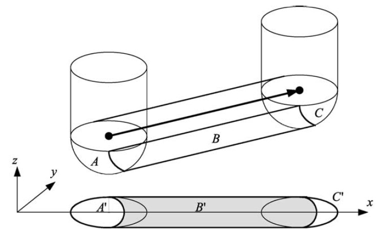
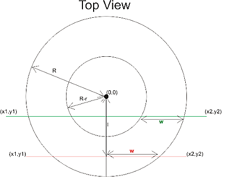
So how do you cut down the z-vectors for each move in the program? For linear moves you can always rotate your coordinate system so it looks like the figure above. The movement is along the x axis, with possibly a simultaneous move in the z-axis. At the beginning of each move (A) and at the end (C) it's very simple, you just calculate the intersection of the relevant z-vectors with a stationary tool at A and C, a kind of 'inverse drop-cutter' idea.

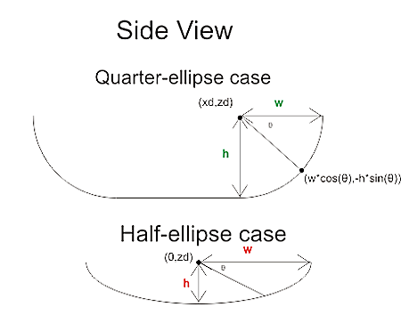
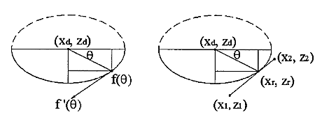
The surface the tool sweeps out during the move itself (B) is more difficult to deal with. The mathematics of the swept surface leads to an equation which most people seem to solve numerically by iteration. I'd like to go through the math/code in a later post (need to learn how to put equations in posts first!).

It's not smart to test all z-vectors in the model against the tool envelope of each move. So like drop-cutter where you are searching for which triangles are under the tool, in z-map you want to know which z-vectors are under the tool envelope. One strategy is simple bucketing, but perhaps if a kd-tree is developed for drop-cutter the same algorithm can be used for z-map.

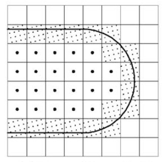
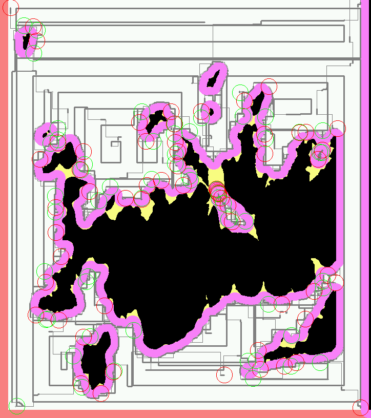
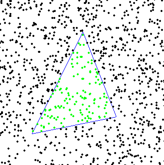
Obviously the z-map has a finite resolution. Increasing the linear resolution by some factor a requires a^2 more z-vectors, storage, and calculations. A better way might be to insert more z-vectors only where they are needed. That's the places on the model where the z-coordinate changes a lot. So here (view from above) for example if you are milling with a cylindrical cutter more z-vectors are needed along the edge of the tool envelope. (I have no idea why they are inserted in a tilted grid-pattern in the above figure...). This potentially leads to much reduced memory/calculation requirements, while still producing a high resolution model. As the simulation progresses there are probably also regions where some densely spaced z-vectors could be removed. Maybe a 'garbage-collector' process could go over the model every now and then and look for flat areas (xy-plane like regions) where less z-vectors are needed and remove them.

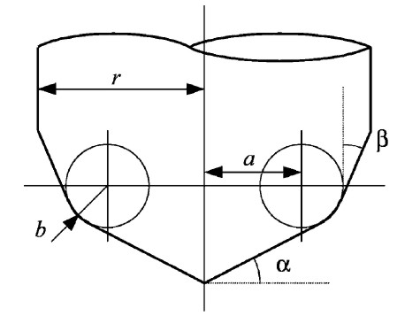
A lot of papers use this APT tool when deriving the equations for machining or simulations. By varying the parameters suitably you get the familiar tool shapes below:

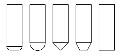
From left to right: Bull-nose/filleted/toroidal, Round/ball-nose/spherical, drill/countersink, tapered, and cylindrical.

My earlier drop-cutter explanations and code only work with the toroidal, spherical, and cylindrical cutters. I'm not sure if it makes sense to write the code for the general APT cutter, or if it's better to optimize for each case (cylindrical and spherical are usually quite easy).

If anyone has made it this far, my sources are the following papers - which are available from me if you ask nicely by email.

Mowing Foam

Dan Egnor sent me this nice example of bitmap-based toolpath generation, or 'pixel mowing'. It's a slightly exaggerated topographic relief of San Francisco machined in tooling board using a very simple 'lawn mowing' toolpath generator.

The explanation of how it works below is mostly Dan's, not mine.

This is the input to the toolpath generator for one of the Z-slices.

black - material which must not be touched
green - to be removed, is safe (at least one tool radius from black)
yellow - remove if possible, is dangerous (within tool radius of black)
purple - has been cleared, is dangerous (machine limits or similar)
white - has been cleared, is safe, is not blue (below)
blue - this spot has been cleared, and is safe, but is within one tool radius of material that needs clearing (green or yellow)

Note that you don't see blue in either "before" or "after" images, it only occurs transiently. (In theory it could show up in "before" as area outside the workpiece.)

And this is the resulting toolpath. Green circles are plunges and red circles are lifts. The thick grey lines represent actual cuts, the thinner lines are rapid feeds.

The basic rule is that the tool *centroid* is only allowed to visit safe areas (green, blue, and white). Green and blue represent work to be done (safe areas that need visiting). Of course, as the tool moves, green changes to blue and white, and (some) yellow changes to purple.

The real trick is in efficiently tracking the "within tool radius of" zones (material to be cut, or material to stay away from). Every pixel keeps a count of how many pixels of each type ("nearby-blocking" or "nearby-cutting") are within one tool radius of that pixel. Whenever a value is changed ( e.g. the simulated tool moves and changes some points from "cut" to "clear"), every counter within the appropriate radius is updated.

That would be rather costly to implement directly, each simulated pixel move would require N^3 updates, if N is the diameter of the tool. Instead those counters are only kept as *differences* between each point and its neighbours. That means changing a point only requires updating the values along the *perimeter* of the radius surrounding that point, meaning that a simulated pixel move only requires N^2 updates, which makes things a lot more tractable (though it still takes the old laptop I use a couple minutes to complete the toolpaths for a 5" x 3" x 1.5" model at 1/256" resolution). Of course this means that the "color state" isn't directly accessible for a random pixel, but must be figured incrementally from neighboring values. Fortunately most operations don't access random pixels.

You would probably not want to cut metal with this kind of algorithm as there is no control over material removal rate or cutting forces, but for foam, tooling-board, or wood it should work ok.

Dan's program is written in C++ and available here (http://svn.ofb.net/svn/egnor/boring/), but it's not well documented.

We are standing by for a video of this kind of cutting!

Mowing tactics

Moving forward with the CAM coding, the sensible thing would probably be to work on mundane things like 2D offset generation, a kd-tree for faster drop-cutter searches, and zigzag-paths from 2D outlines... There's again been some talk about open-source CAM on cnczone, but not much in terms of results or actual descriptions or implementations of toolpath algorithms.

Anyway, here's something more fun than the traditional computational geometry problems I referred to above. It's lawn-mowing tactics, or how do you program the circular robot to mow the red pixels while not cutting too many of them at a time. This is a slightly improved version of my earlier trial. This one considers a number of angles in all directions for each move. From these moves the ones that cut away a suitable amount of material are selected. Additionally I've introduced a cost function for changing direction, it should be easier for the cutter to continue traveling in approximately the same direction than to do abrupt turns. In spite of this, about half-way through the cutter reverses direction...This is obviously done with a bitmap representing the grass to be mowed, but I wonder if it would be better to try to do it more exactly: represent the boundaries of the grass with lines and arcs. A variable step-length also seems like a good idea, on long straight bits the cutter should be able to move in one go as far as it goes.

Drop-Cutter in C# - v2

I think I've found the problems with my C# drop-cutter algorithm. The first bug was a trivial one where in the edge-test the rotation of the segment-under-test was messed up. The second one was not the facet-test itself but incorrect surface normal data. There's something going on that makes pre-calculated surface normal data not 'stick' correctly to the triangle object for later use. So here I'm re-calculating the normal data again just before the facet test.

The next step is to speed up things with a smarter kd-tree based search for which triangles are under the cutter. I've added bounding-boxes to the Cutter and Triangle classes. Running the above example the DropCutter function is called a total of 4735000 times, and of those only less than 5%, or 236539 to be exact, are useful calls, i.e. the triangle bounding box intersects the cutter bounding box, which means there's a chance that we are contacting the cutter against the triangle. The idea with the kd-tree then is to pre-search for triangles under the cutter to make less of those (supposedly expensive) redundant calls to DropCutter.

On my T5600 processor machine the above example runs in about 5 seconds. (1894 triangles, about 4.7 Million calls to DropCutter of which ca 240k calculate something). I've made a list of useful CAM-related things to work on: CAMToDo.

Drop-Cutter in C#

I've now ported my Matlab work on Drop-Cutter to C#. It can load an ASCII STL file and then run the drop cutter algorithm. Not trying to take too much on in the beginning, here's an example of the output with only two triangles as input 🙂 not quite there yet! (who can spot what's wrong?)

I'll do some nicer demos when I've found the problem. The algorithm runs significantly faster in C# compared to Matlab - and this is without a kd-tree or bucket strategy for finding triangles under the cutter. I've also watched and read some tutorials on threading (threading wrt. to computers, not machining!). This is an algorithm that should scale well on modern multi-core processors (have a few worker-threads running drop-cutter on different regions of the model).

An STL Tux

Together with another Anders (from Sweden) I've worked a little bit on some C# code for rendering stuff in OpenGL. The idea is to put together a basic framework where CAD/CAM ideas and algorithms can be tested. Above one of the first useful screenshots where I've rendered an STL file with about 22k triangles.

The code needs to be cleaned up and made all object-oriented and nice, but after that it should not be hard to test the Drop-Cutter algorithm and generate some raster-finish paths.

I've also been reading a 2004 paper by Yau et al. which explains the drop-cutter algorithm for an APT tool. I'm not very interested in the tapered cutters - but that can be added later if needed. What's more interesting in the paper is a kd-tree approach for finding out which triangles are under the 'shadow' of the cutter.

The idea is that it's not necessary to test against all triangles, only those that are under the cutter. Since the circular cutter and the triangles are differently shaped, Yau et al. start by approximating both cutter and triangles with rectangles. So they generate rectangular bounding boxes around each triangle and also around the cutter. The task then is for a given position of the cutter to find which bounding-boxes(triangles) intersect it. I understand this is a variant of what's called an orthogonal range search in computer science.

If anyone with a good understanding of kd-trees and/or range-searching is willing to help with a C# implementation I'd be glad to send over the Yau et al. pdf!

Drop cutter might work!

Here's the first indication that my drop cutter algorithms(vertex, facet, edge) might work! I'm dropping down a toroidal cutter C(0.5, 0.125) towards a model consisting of a half-sphere sitting on a plane. The CL points are in magenta with cyan lines between them. 382 triangles in total. The code has no optimizations, so at each x,y position we check against all triangles.

Here's another one with about 1800 triangles, and with the points more densely sampled in the Y-direction. (click for slightly higher resolution version)

These still pictures are not nearly as convincing as a moving animation - so I will have to do that next with a more complex model. Stay tuned...

Drop Cutter 3/3: Edge Test

The third and final test in the drop cutter algorithm is to drop the cutter down so it touches an edge. The vertex and facet tests were quite easy, but this one requires a bit of calculations. I'm following Chuang2002.
To simplify things we first translate the tool in the (x, y) plane to (0, 0), and then rotate the edge we are testing against so that it lies along the x-axis and is below the cutter (or on top of the x-axis). The distance from the edge to (0, 0) is l.

Now we imagine a vertical plane through the edge and slice the cutter with that plane. There are two cases, depending on l.

If R-r>l we are cutting with a plane (green) that results in an intersection that has two quarter ellipses at the sides and a flat part in the middle. These ellipses have centers with
xd = +/- sqrt( (R-r)^2 - l^2 )

The other case is shown with a red line: if
R-r<=l<R
the intersection of the cutter will be a half ellipse centered at xd=0.
In both cases the curved part of the intersection is described by
f(theta) = (w*cos(theta) , h*cos(theta) ) where 0<theta<pi
h and w, the height and width of the ellipse are given by

  • quarter-ellipse case:
    • h=r
    • w=sqrt(R^r - l^2) - sqrt( (R-r)^2 - l^2 )
  • half -ellipse case:
    • h=sqrt( r^2 -(l-(R-l))^2 )
    • w=sqrt(R^2-l^2)

Now that the geometry is clear we can have the edge contact the intersection. That happens at a point where the tangents("slopes") are equal. A tangent vector to the ellipse is given by
f'(theta) = (-w*sin(theta) , -h*cos(theta) )
which can be equated with the slope of the line:
w*sin(theta) / h*cos(theta) = (x1-x2)/(z1-z2)
and we find the angle theta of our CC point:
theta = atan( h*(x1-x2)/w*(z1-z2))
(z1=z2 is a trivial special case not handled here)

The CC point is now given by
xc = xd +/- abs(w*cos(theta))
which should be checked if it lies between x1 and x2. If it does we are contacting the edge, and we can calculate the z-coordinate of the CC point as:
zc = ((xc-x1)/(x2-x1))*(z2-z1) +z1
and finally that leads us to the correct cutter height
ze = zc + abs(h*sin(theta)) - r

Now I need to put all these tests together and find a way of importing STL files into matlab. That way I can begin to test if/how my drop cutter algorithm works!

There's still a lot to do before I have a set of algorithms for basic 3-axis toolpath creation: "push-cutter" a 2D version of drop cutter, 2D line/arc? offsets, zigzag paths, STL-slice with plane, z-buffer simulation of stock material, to name a few things...

An emergent spiral

Most conventional CAM algorithms are geometry-based. They create toolpaths that are usually parallel to either the coordinate axes ('zigzag'-paths) or to the part contour (contour-parallel, or spiral paths). One problem with this geometry-based stuff is that you don't take into account the cutting forces. The algorithm has no idea about how much material is removed while the tool is moving. A quick patch is to run a cutting simulation after the path is created and adapt the feedrate for constant material removal rate (MRR).

Another option is to base the toolpath algorithm on a stock model. Then you know the shape of the stock at all times and you can control the MRR or cutter engagement angle. To quickly test how this could work I made a small test in matlab.

The cutter (green circle) is moved around by some rules, and cut's the red pixels as it travels over them. Cut pixels are drawn in blue. The cutter is moved around in discrete steps in some direction, and you're only allowed to cut a certain number of pixels per move. The tricky part is coming up with the rules for our 'lawn-mower' robot. Now I'm using a simple idea: If the past move was made at an angle alfa, try to take the next step in the same direction, but if that's not possible increase alfa until the MRR goes down to some preset value.

This idea will need refinement so that the robot can cope with walls, can do cutting in only one direction (climb vs. conventional) etc. etc., but this seems like a promising and fun start!

Point in triangle test

The facet test I wrote about yesterday needs a 'point in triangle' test to determine if the found CC point lies within the given triangle and we should thus care about the ze value the algorithm determined, or if the CC point is outside, and we can skip to the next test/triangle.

I wrote a function isright(p1,p2,p) which tells me whether the point p is right or left of the line from p1 to p2. The triangle test isinside(p1,p2,p3,p) uses this function three times:
t1 = isright(p1,p2,p);
t2 = isright(p3,p1,p);
t3 = isright(p2,p3,p);

and if t1, t2, t3 all have the same sign then p is inside the triangle.

If I add this function to the facet test, I can determine which of the CC points in the plane containing the triangle are within the triangle:


here the dashed line indicates the z-axis.

I'm a little concerned that this works with the projection of the triangle onto the xy-plane. But maybe that isn't a problem because triangles with horizontal normals are special cases anyway. I also haven't yet looked at the rounding/on-edge problems Julian talks about.

I wish the third and final part of this story, the edge-test, was as simple as the vertex and facet tests! At least so far I haven't found a really simple algorithm for the edge-test in the literature (I'm reading Hwang1998 and Chuang2002). Anyone know more about this? please comment below!