Better adaptive waterline

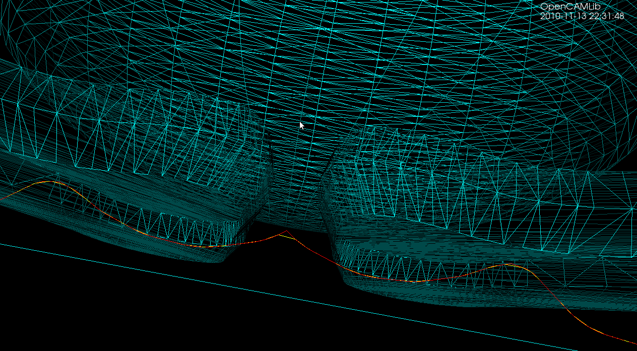
Previously the flat() predicate looked only at the number of intervals contained in a fiber when deciding where to insert new fibers in the adaptive waterline algorithm. Here I've borrowed the same flat() function used in adaptive drop-cutter which computes the angle between subsequent line-segments(yellow), and inserts a new fiber(cyan) if the angle exceeds some pre-set threshold.

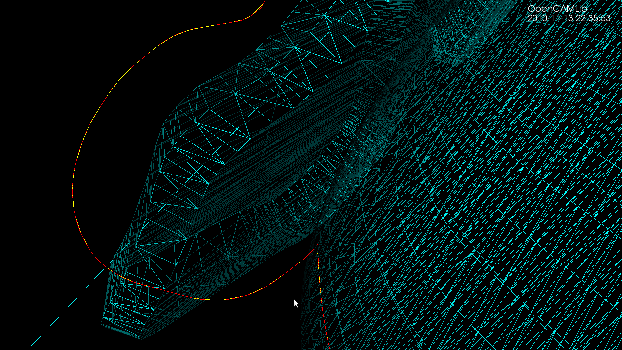
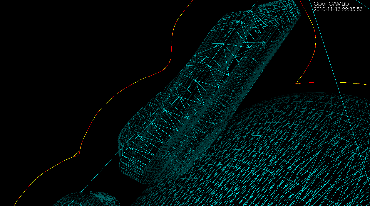
This works on the larger Tux model also. However, there's no free lunch: the uniformly sampled waterline (yellow) runs in about 2 s (using OpenMP on a dual-core machine), while the adaptively sampled waterline takes around 30s to compute (no OpenMP).

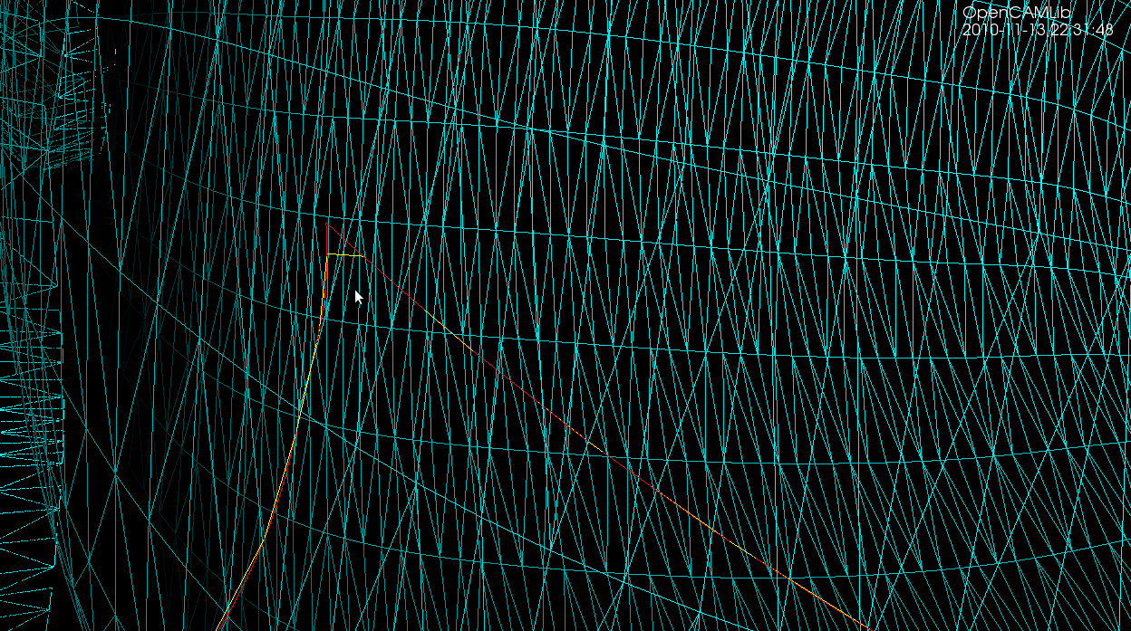
The difference between the adaptive (red) and the uniformly sampled (yellow) waterlines is really only visible when zooming in on sharp corners or other details. Compare this to adaptive drop-cutter.


EMC2 upgrade

I've upgraded Ubuntu and EMC2 on the Atom 330 machine I have for controlling the lathe. The Atom 330 is a dual-core chip, but with Hyper Threading the OS can see four cores. That's not good for real-time performance, so the first thing I did was turn off HT from the BIOS. Next I did a distribution upgrade to 10.04LTS which downloaded about 1 Gig in an estimated 9 minutes (2Mb/s is OK I guess...). I then used the emc2-install script which installs the real-time kernel and emc2, and finally I edited /boot/grub/menu.lst by adding "isolcpus=1" on the kernel line. This reserves one cpu core for real-time and the other for non-real-time tasks. Without "isolcpus=1" the latency-test jitter values were easily 10k and more with a light load on the machine. With one core dedicated to real-time the jitter numbers start out at around 4k at light load and double to 7-8k under heavy load.

Here are some selected screenshots:

Next stop is getting the X and Z servos moving, as well as the hefty 2 kW spindle servo.

On the density of doubles and floats

With finite precision numbers, if you take a small number eps, there comes a point when x == x + eps. Here's some code that figures out when that happens:

double epsD(double x) {
    double r;
    r = 1000.0;
    while ( x < (x + r) )
        r = r / 2.0;
    return ( 2.0 * r );
}

With x around one the resolution limit is roughly at 1e-16 for doubles, and 1e-7 for floats. The top data points show how the relative accuracy stays constant, so at x=1e7 the resolution is only about eps=1 for floats.

Thinking about CAD/CAM related stuff, if you have a fancy top of the line CNC-machine with the longest axis x=1000mm and a theoretical accuracy of one micron, or 0.001mm, then we're at the point where we really should use doubles (which are slower, but how much slower?).

python source for plotting the figure: epsplot.py.tar

Waterline problem

I was trying to work on a new adaptive waterline feature, but ended up uncovering an old existing problem/bug with waterline. I think it has to be a problem in either building the weave from the fibers, or constructing the planar embedding of the weave.

The yellow waterline should obviously be a smooth loop around the outside of the weave (red/green fibers) and not a zigzag journey back and forth... 🙁

Update: this is better now:

Update2: here's a figure where new fibers (red and green) are inserted adaptively where the shape of the waterline changes most. There's something wrong with building the planar embedding for this weave, so no yellow adaptive waterline path yet...

Update3: some progress at last (fixed a bug in adaptive drop-cutter at the same time):


Qt and OpenGL test

It looks like there is no efficient way of updating (adding and removing) triangles in a polydata-surface in VTK, so for the cutting-simulation I am looking at other visualization options. Despite all the tutorials and documentation out there on the interwebs it always takes about two hours to get these "Hello World" examples running...

Download a zip-file with the source and cmake file: (This compiles and runs on Ubuntu 10.04LTS) qtopengl