The plan was to run at a nice and even 5:40/km pace to finish in 4 hours, but after feeling OKish for the first two laps out of four, suddenly I felt overheated and dehydrated and stepped off after 22km.
The pace on laps 1 and 2 was exactly as planned, 27:30 for the first 5k (5:30/km), 28:25 for 5-10km (5:41/km), 28:10 for the third 5k from 10 to 15k (5:38/km) and 28:53 for 15-20k (5:47/km). I was on track to run that four hour marathon, but somehow in the warm and windy weather wasn't getting enough water, energy or, something else. Oh well, there's always next year...
It's probably much easier to figure out the connections from the diagram below than to browse the text files. The square wave, which has a frequency proportional to the temperature, comes in on parallel port pin-13, and is connected to an encoder. The encoder has a velocity output which will be equal to the frequency of the square wave in Hz. This frequency is used as the feedback for a PID-component which compares the measured frequency against a set-point which is taken from a pyvcp slider. The pid output is used as an input to a pwm-generator, whose output needs an inverter, since the pwm-amplifier is active-low. The PWM is output on parallel port pin 9.
I wish there was a tool which would draw these HAL/pyVCP diagrams automagically from the source files. There is some work in that direction already: crapahalic and HAL with gschem.
With a bucketing-scheme for nearest-neighbour search in expected time O(1) this voronoi-diagram generation for 100k sites in the [0,1] unit square now runs in 30 s, i.e. it takes about 0.3 ms to insert one point.
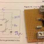
I made two small circuits today for temperature control of the extruder head on a reprap type 3D printer. The idea is to control the temperature, which needs to be somewhere between 200 and 240 C I think, using EMC2 and two parallel port pins.
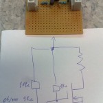
The first circuit is based on the 555 and produces a square waveform with variable frequency depending on the resistance of a thermistor. At room temperature the thermistor resistance is 100 kOhms and the output frequency is below 1 Hz, and when the temperature is suitable for extrusion the thermistor resistance is about 200 Ohms which produces an output frequency of around 25-30 Hz. If the EMC2 base-thread runs with a 50 us period then it should be possible to record the frequency of this square wave using an input pin on the parallel port with an accuracy of roughly 1/500 (half a degree C?), which should suffice.
Testing the heating side of things, a wire with about 6 ohms of resistance wrapped around the extruding head, showed that a suitable DC voltage is around 8 V and produces a current of 1.3 A. The idea is to use a HAL PWM-generator to drive the base of a 337 transistor which drives the gate of an IRF610 FET that controls the current through the heating wire. By adjusting the PWM duty cycle it should be possible to control the temperature using a PID controller based on the temperature measurement.
The algorithm works by incrementally constructing the diagram while adding the point-generators one by one. This initial configuration is used at the beginning:
The diagram will be correct if new generator points are placed inside the orange circle (this way we avoid edges that extend to infinity). Once about 500 randomly chosen points are added the diagram looks like this:
Because of floating-point errors it gets harder to construct the correct diagram when more and more points are added. My code now crashes at slightly more than 500 generators (due to an assert() that fails, not a segfault - yay!). It boils down to calculating the sign of a 4-by-4 determinant, which due to floating-point error goes wrong at some point. That's why the Sugihara-Iri algorithm is based on strictly preserving the correct topology of the diagram, and in fact they show in their papers that their algorithm doesn't crash when a random error is added to the determinant-calculations, and it even works (in some sense) when the determinant calculation is completely replaced by a random number generator. Their 1992 paper constructs the diagram for one million generators using 32-bit float
numbers, while my naive attempt using double here crashes after 535 points... some work to do still then!
Note how within one voronoi-region the offset is determined by the associated generator (a line, point, or arc). It's very easy to figure out the offset within one region: points and arcs have circular offsets, while lines have line offsets. The complete offset path is a result of connecting the offset from one region with the next region.
I've run actively this year from week 13, which means 34 weeks of running/jogging so far. Or an average of 29.56km per week. Weeks 15, 19, and 37 were the low points with only 5-6 km completed (week 37 I had a fever). Week 29 (55k total) is one of the most active with a 24k long run(in central park, IIRC) in the beginning of the week, some short runs in the middle, and the Jakob half-marathon on the weekend.
At 30km/week the total should land on roughly 1200 km for this year.
There's some peer pressure on signing up for the Finlandia langlauf in February... we'll see if that happens or not.
Legs still feel a bit heavy from Sunday. This week is supposed to be a lot easier than last week, and next week is just light jogging before the D-day...
There was an uphill about 2/3rds into the last repeat which causes a jump in the HR-trace.